Chapter 2: Variables

A variable is a characteristic that exhibits detectable changes, either regionally or temporally. Implicit in this concept of change is influence by something else: Newtonian dynamics show us that movement in itself does not imply an external force -- change in movement does. Thus scientists are seldom concerned with a single variable; more often we seek patterns among variables. This chapter focuses on one variable at a time, thereby setting the stage for considerations in the next chapter of relationships among variables.

Variables, measurements, and quantification are related components of the foundation of science. Characterizing a variable requires measurements, and measurements require prior quantification. Each variable has an associated measurement type:

•     Nominal measurements classify information and count the frequency of observations within each class. An example is tabulation of the numbers of protons and neutrons in an atom.

•     Ordinal measurements specify order, or relative position. Ordinal scales may be objectively determined (e.g., the k, l, and m electron shells), subjectively determined but familiar (e.g., youth, young adult, adult, old age), or subjectively invented for a particular experiment (e.g., social science often uses scales such as this: strongly agree (+2), agree (+1), not sure (0), disagree (-1), strongly disagree (-2)).

•     Interval and ratio scales permit measurements of distance along a continuum, with determinable distance between data. The scales involve either real (fractional) or integer (counting) numbers. They differ in that only ratio scales have a true, or meaningful, zero, permitting determination of ratios between data measurements. For example, temperatures are measured with an interval scale, whereas length is a ratio scale. To refer to one temperature as twice that of another is pointless, whereas it is valid to say that one object is twice as long as another.

The initial quantification of any variable is challenging, for we seek a scale that is both measurable and reliable. Soon, however, that quantification is taken for granted. Finding a way to quantify some variable tends to be more of a problem in the social sciences than in the physical sciences.

*     *     *

Statistics

Statistics are pattern recognition transformed, from a qualitative guess about what may be, into a quantitative statement about what probably is.

A decade ago, scientific statistics usually required either complex number crunching or simplifying approximations. Since then, computers have revolutionized our approach to statistics. Now standard statistical techniques are available on most personal computers by simply choosing an option, and programs for even the most sophisticated statistical techniques are available from books such as Numerical Recipes [Press et al., 1988]. With easy access comes widespread misuse; one can use various statistical routines without learning their assumptions and limitations.

Statistics help us both to solve single-variable problems (this chapter) and to accomplish multivariate pattern recognition (next chapter). Neither chapter is a substitute for a statistics course or statistics book; no proofs or derivations are given, and many subjects are skipped. Statistics books present the forward problem of looking at the statistical implications of each of many groups of initial conditions. The scientist more often faces the inverse problem: the data are in-hand, and the researcher wonders which of the hundreds of techniques in the statistics book is relevant.

Efficiency is a key to productive science. Statistics and quantitative pattern recognition increase that efficiency in many ways: optimizing the number of measurements, extracting more information from fewer observations, detecting subtle patterns, and strengthening experimental design. Statistics may even guide the decision on whether to start a proposed experiment, by indicating its chance of success. Thus, it is a disservice to science to adopt the attitude of Rutherford [Bailey, 1967]: “If your experiment needs statistics, you ought to have done a better experiment.”

These two chapters introduce some of the statistical methods used most frequently by scientists, and they describe key limitations of these techniques. Rather than an abridged statistics book, the chapters are more an appetizer, a ready reference, an attempt at demystifying a subject that is an essential part of the scientific toolbox.

*     *     *

Errors

All branches of science use numerical experimental data, and virtually all measurements and all experimental data have errors -- differences between measurements and the true value. The only exceptions that I can think of are rare integer data (e.g., how many of the subjects were male?); real numbers are nearly always approximate. If a measurement is repeated several times, measurement errors are evident as a measurement scatter. These errors can hide the effect that we are trying to investigate.

*     *     *

Errors do not imply that a scientist has made mistakes. Although almost every researcher occasionally makes a mathematical mistake or a recording error, such errors are sufficiently preventable and detectable that they should be extremely rare in the final published work of careful scientists. Checking one’s work is the primary method for detecting personal mistakes. Scientists vary considerably in how careful they are to catch and correct their own mistakes.

How cautious should a scientist be to avoid errors? A scientist’s rule of thumb is that interpretations can be wrong, assumptions can be wrong, but there must be no data errors due to mistakes. The care warranted to avoid errors is proportional to the consequences of mistakes. A speculation, if labeled as such, can be wrong yet fruitful, whereas the incorrect announcement of a nonprescription cure for cancer is tantamount to murder.

Physicist George F. Smoot set a standard of scientific caution: for 1 1/2 years he delayed announcement of his discovery of heterogeneities in the background radiation of the universe, while his group searched avidly for any error in the results. He knew that the discovery provided critical confirmation of the Big Bang theory, but he also knew that other scientists had mistakenly claimed the same result at least twice before. Consequently, he made the following standing offer to members of his research team: to anyone who could find an error in the data or data analysis, he would give an air ticket to anywhere in the world. [5/5/92 New York Times]

I imagine that he was also careful to emphasize that he was offering a round-trip ticket, not a one-way ticket.

Both scientists and non-scientists have recognized the constructive role that error can play:

“Truth comes out of error more readily than out of confusion.” [Francis Bacon, 1620]

“The man who makes no mistakes does not usually make anything.” [Phelps, 1899]

Incorrect but intriguing hypotheses can be valuable, because the investigations that they inspire may lead to a discovery or at least show the way toward a better hypothesis (Chapter 7). Humphrey Davy [1840] said, “The most important of my discoveries have been suggested by my failures.” More rarely, incorrect evidence can inspire a fruitful hypothesis: Eldredge and Gould’s [1972] seminal reinterpretation of Darwinian evolution as punctuated equilibrium initially was based on inappropriate examples [Brown, 1987].

Errors are most likely to be detected upon first exposure. Once overlooked, they become almost invisible. For example, if an erroneous hypothesis passes initial tests and is accepted, it becomes remarkably immune to overthrow. 

“One definition of an expert is a person who knows all the possible mistakes and how to avoid them. But when we say that people are ‘wise’ it’s not usually because they’ve made every kind of mistake there is to make (and learned from them), but because they have stored up a lot of simulated scenarios, because their accumulated quality judgments (whether acted upon or not) have made them particularly effective in appraising a novel scenario and advising on a course of action.” [Calvin, 1986]

*     *     *

Errors arise unavoidably: unrecognized variations in experimental conditions generate both so-called ‘random’ errors and systematic errors. The researcher needs to know the possible effects of errors on experimental data, in order to judge whether or not to place any confidence in resulting conclusions. Without knowledge of the errors, one cannot compare an experimental result to a theoretical prediction, compare two experimental results, or evaluate whether an apparent correlation is real. In short, the data are nearly useless.

*     *     *

Precision > Accuracy > Reliability

The terms precision, accuracy, reliability, confidence, and replicatability are used interchangeably by most non-scientists and are even listed by many dictionaries as largely synonymous. In their scientific usage, however, these terms have specific and important distinctions.

Errors affect the precision and accuracy of measurements. Precision is a measure of the scatter, dispersion, or replicatability of the measurements. Low-precision, or high-scatter, measurements are sometimes referred to as noisy data. Smaller average difference between repeat (replicate) measurements means higher precision. For example, if we measure a sheet of paper several times with a ruler, we might get measurements such as 10.9", 11.0", 10.9", and 11.1". If we used a micrometer instead, we might get measurements such as 10.97", 10.96", 10.98", and 10.97". Our estimates show random variation regardless of the measuring device, but the micrometer gives a more precise measurement than does the ruler. If our ruler or micrometer is poorly made, it may yield measurements that are consistently offset, or systematically biased, from the true lengths. Accuracy is the extent to which the measurements are a reliable estimate of the ‘true’ value. Both random errors and systematic biases reduce accuracy.

Reliability is a more subjective term, referring usually to interpretations but sometimes to measurements. Reliability is affected by both precision and accuracy, but it also depends on the validity of any assumptions that we have made in our measurements and calculations. Dubious assumptions, regardless of measurement precision and accuracy, make interpretations unreliable.

*     *     *

Random and Systematic Errors

Random errors are produced by multiple uncontrolled and usually unknown variables, each of which has some influence on the measurement results. If these errors are both negative and positive perturbations from the true value, and if they have an average of zero, then they are said to affect the precision of replicate measurements but they do not bias the average measurement value.

If the errors average to a nonzero value, then they are called systematic errors. A constant systematic error affects the accuracy but not the precision of measurements; a variable systematic error affects both accuracy and precision. Systematic errors cause a shift of individual measurements, and thus also of the average measured value, away from the true value. Equipment calibration errors are a frequent source of systematic errors. Inaccurate calibration can cause all values to be too high (or low) by a similar percentage, a similar offset, or both. An example of a systematic percentage bias is plastic rulers, which commonly are stretched or compressed by about 1%. An example of an offset bias is using a balance without zeroing it first. Occasionally, systematic errors may be more complicated. For example, a portable alarm clock may be set at a slightly incorrect time, run too fast at first, and run too slowly when it is about ready for rewinding.

Both random and systematic errors are ubiquitous. In general, ‘random errors’ only appear to be random because we have no ability to predict them. If either random or systematic errors can be linked to a causal variable, however, it is often possible to remove their adverse effects on both precision and accuracy.

One person’s signal is another person’s noise, I realized when I was analyzing data from the Magsat satellite. Magsat had continuously measured the earth’s magnetic field while orbiting the earth. I was studying magnetism of the earth’s crust, so I had to average out atmospheric magnetic effects within the Magsat data. In contrast, other investigators were interested primarily in these atmospheric effects and were busily averaging out crustal ‘contamination.’

Random errors can be averaged by making many replicate, or repeat, measurements. Replicate measurements allow one to estimate and minimize the influence of random errors. Increasing the number of replicate measurements allows us to predict the true value with greater confidence, decreasing the confidence limits or range of values within which the true value lies. Increasing the number of measurements does not rectify the problem of systematic errors, however; experimental design must anticipate such errors and attenuate them.

*     *     *

Representative Sampling

Most experiments tackle two scientific issues -- reducing errors and extrapolating from a sample to an entire population -- with the same technique: representative sampling. A representative sample is a small subset of the overall population, exhibiting the same characteristics as that population. It is also a prerequisite to valid statistical induction, or quantitative generalization. Nonrepresentative sampling is a frequent pitfall that is usually avoidable. Often, we seek patterns applicable to a broad population of events, yet we must base this pattern recognition on a small subset of the population. If our subset is representative of the overall population, if it exhibits similar characteristics to any randomly chosen subset of the population, then our generalization may have applicability to behavior of the unsampled remainder of the population. If not, then we have merely succeeded in describing our subset.

Representative sampling is essential for successful averaging of random errors and avoidance of systematic errors, or bias. Random sampling achieves representative sampling. No other method is as consistently successful and free of bias. Sometimes, however, random sampling is not feasible. With random sampling, every specimen of the population should have an equal chance of being included in the sample. Every specimen needs to be numbered, and the sample specimens are selected with a random number generator. If we lack access to some members of the population, we need to employ countermeasures to prevent biased sampling and consequent loss of generality. Stratification is such a countermeasure.

Stratification does not attempt random sampling of an entire population. Instead, one carefully selects a subset of the population in which a primary variable is present at a representative level. Stratification is only useful for assuring representative sampling if the number of primary variables is small. Sociologists, for example, cannot expect to find and poll an ‘average American family’. They can, however, investigate urban versus rural responses while confining their sampling to a few geographical regions, if those regions give a stratified, representative sample of both urban and rural populations.

For small samples, stratification is actually more effective in dealing with a primary variable than is randomization: stratification deliberately assures a representative sampling of that variable, whereas randomization only approximately achieves a representative sample. For large samples and many variables, however, randomization is safer. Social sciences often use a combination of the two: stratification of a primary variable and randomization of other possible variables [Hoover, 1988]. For example, the Gallup and Harris polls use random sampling within a few representative areas.

In 1936, the first Gallup poll provided a stunning demonstration of the superiority of a representative sample over a large but biased sample. Based on polling twenty million people, the Literary Digest projected that Landon would defeat Roosevelt in the presidential election. The Literary Digest poll was based on driver’s license and telephone lists; only the richer segment of the depression-era population had cars or telephones. In contrast, George Gallup predicted victory for Roosevelt based on a representative sample of only ten thousand people.

The concept of random sampling is counterintuitive to many new scientists and to the public. A carefully chosen sample seems preferable to one selected randomly, because we can avoid anomalous, rare, and unusual specimens and pick ones exhibiting the most typical, broad-scale characteristics. Unfortunately, the properties of such a sample probably cannot be extrapolated to the entire population. Statistical treatment of such data is invalid. Furthermore, sampling may be subconsciously biased, tending to yield results that fulfill the researcher’s expectations and miss unforeseen relationships (Chapter 6). Selective sampling may be a valid alternative to random sampling, if one confines interpretations to that portion of the population for which the sample is a representative subset.

Even representative sampling cannot assure that the results are identical to the behavior of the entire population. For example, a single coin flip, whether done by hand or by a cleverly designed unbiased machine, will yield a head or a tail, not 50% heads and 50% tails. The power of random sampling is that it can be analyzed reliably with quantitative statistical techniques such as those described in this chapter, allowing valid inferences about the entire population. Often these inferences are of the form ‘A probably is related to B, because within my sample of N specimens I observe that the A_i are correlated with B_i.’

*     *     *

Replication and Confirmation

The terms replicatability and reproducibility are often used to refer to the similarity of replicate measurements; in this sense they are dependent only on the precision of the measurements. Sometimes replicatability is used in the same sense as replication, describing the ability to repeat an entire experiment and obtain substantially the same results. An experiment can fail to replicate because of a technical error in one of the experiments. More often, an unknown variable has different values in the two experiments, affecting them differently. In either case the failure to replicate transforms conclusions. Identifying and characterizing a previously unrecognized variable may even eclipse the original purpose of the experiments.

Replication does not imply duplication of the original experiment’s precision and accuracy. Indeed, usually the second experiment diverges from the original in design, in an attempt to achieve higher precision, greater accuracy, or better isolation of variables. Some [e.g., Wilson, 1952] say that one should not replicate an experiment under exactly the same conditions, because such experiments have minor incremental information value. Exact replication also is less exciting and less fundamental than novel experiments.

If the substantive results (not the exact data values but their implications) or conclusions of the second experiment are the same as in the first experiment, then they are confirmed. Confirmation does not mean proved; it means strengthened. Successful replication of an experiment is a confirmation. Much stronger confirmation is provided by an experiment that makes different assumptions and different kinds of measurements than the first experiment, yet leads to similar interpretations and conclusions.

In summary, precision is higher than accuracy, because accuracy is affected by both precision and systematic biases. Accuracy is higher than reliability, because reliability is affected not just by measurement accuracy but also by the validity of assumptions, simplifications, and possibly generalizations. Reliability is increased if other experiments confirm the results.

*     *     *

Probability

Probability is a concern throughout science, particularly in most social sciences, quantum physics, genetics, and analysis of experiments. Probability has a more specific meaning for mathematicians and scientists than for other people. Given a large number of experiments, or trials, with different possible outcomes, probability is the proportion of trials that will have one type of outcome. Thus the sum of probabilities of all possible outcomes is one.

Greater probability means less uncertainty, and one objective of science is to decrease uncertainty, through successful prediction and the recognition of orderly patterns. Induction (Chapter 3), which is a foundation of science, is entirely focused on determining what is probably true. Only by considering probability can we evaluate whether a result could have occurred by chance, and how much confidence to place in that result.

“Looking backwards, any particular outcome is always highly improbable” [Calvin, 1986]. For example, that I am alive implies an incredibly improbable winning streak of birth then reproduction before death that is several hundred million years long. Yet I do not conclude that I probably am not alive. The actual result of each trial will be either occurrence or nonoccurrence of a specific outcome, but our interest is in proportions for a large number of trials.

The most important theorem of probability is this: when dealing with several independent events, the probability of all of them happening is the product of the individual probabilities. For example, the probability of flipping a coin twice and getting heads both times is 1/2•1/2=1/4; the chance of flipping a coin and a die and getting a head plus a two is 1/2•1/6=1/12. If one has already flipped a coin twice and gotten two heads, the probability of getting heads on a third trial and thus making the winning streak three heads in a row is 1/2, not 1/2•1/2•1/2=1/8. The third trial is independent of previous results.

Though simple, this theorem of multiplicative probabilities is easy to misuse. For example, if the probability of getting a speeding ticket while driving to and from work is 0.05 (i.e., 5%) per round trip, what is the probability of getting a speeding ticket sometime during an entire week of commuting? The answer is not .05•.05•.05•.05•.05=.0000003; that is the probability of getting a speeding ticket on every one of the five days. If the question is expressed as “what is the probability of getting at least one speeding ticket”, then the answer is 1-0.95⁵=0.226, or 1 minus the probability of getting no speeding tickets at all.

Often the events are not completely independent; the odds of one trial are affected by previous trials. For example, the chance of surviving one trial of Russian roulette with a 6-shot revolver is 5/6; the chance of surviving two straight trials (with no randomizing spin of the cylinders between trials) is 5/6•4/5=2/3.

Independence is the key to assuring that an undesirable outcome is avoided, whether in a scientific research project or in everyday life. The chance of two independent rare events occurring simultaneously is exceedingly low. For example, before a train can crash into a station, the engineer must fail to stop the train (e.g., fall asleep) and the automatic block system must fail. If the chance of the first occurring is 0.01 and the chance of the second occurring is 0.02, then the chance of a train crash is the chance of both occurring together, or 0.01•0.02=0.0002. The same strategy has been used in nuclear reactors; as I type this I can look out my window and see a nuclear reactor across the Hudson River. For a serious nuclear accident to occur, three ‘independent’ systems must fail simultaneously: primary and secondary cooling systems plus the containment vessel. However, the resulting optimistic statements about reactor safety can be short-circuited by a single circumstance that prevents the independence of fail-safes (e.g., operator panic misjudgments or an earthquake).

Entire statistics books are written on probability, permitting calculation of probabilities for a wide suite of experimental conditions. Here our scope is much more humble: to consider a single ‘probability distribution function’ known as the normal distribution, and to determine how to assess the probabilities associated with a single variable or a relationship between two variables.

*     *     *

Sampling Distribution for One Variable

Begin with a variable which we will call X, for which we have 100 measurements. This dataset was drawn from a table of random normal numbers, but in the next section we will consider actual datasets of familiar data types. Usually we have minimal interest in the individual values of our 100 (or however many) measurements of variable X; these measurement values are simply a means to an end. We are actually interested in knowing the true value of variable X, and we make replicate measurements in order to decrease the influence of random errors on our estimation of this true value. Using the term ‘estimation’ does not imply that one is guessing the value. Instead ‘estimation’ refers to the fact that measurements estimate the true value, but measurement errors of some type are almost always present.

Even if we were interested in the 100 individual values of X, we face the problem that a short or prolonged examination of a list of numbers provides minimal insight, because the human mind cannot easily comprehend a large quantity of numbers simultaneously. What we really care about is usually the essence or basic properties of the dataset, in particular:

• what is the average value?
• what is the scatter?
• are these data consistent with a theoretically predicted value for X?
• are these data related to another variable, Y?

With caution, each of the first three questions can be described with a single number, and that is the subject of this chapter. The engaging question of relationship to other variables is discussed in Chapter 3.

Histograms

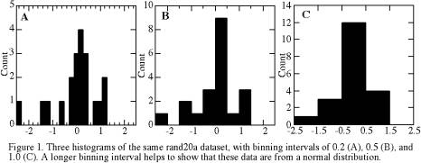
The 100 measurements of X are more easily visualized in a histogram than in a tabulation of numbers. A histogram is a simple binning of the data into a suite of adjacent intervals of equal width. Usually one picks a fairly simple histogram range and interval increment. For example, our 100 measurements range from a minimum of -2.41 to a maximum of 2.20, so one might use a plot range of -2.5 to 2.5 and an interval of 0.5 or 1.0, depending on how many data points we have. The choice of interval is arbitrary but important, as it affects our ability to see patterns within the data. For example, Figure 1 shows that for the first 20 values of this dataset:

• an interval of 0.2 is too fine, because almost every data point goes into a separate bin. The eye tends to focus mainly on individual data points rather than on broad patterns, and we cannot easily see the relative frequencies of values.

• an interval of 0.5 or 1.0 is good, because we can see the overall pattern of a bell-shaped distribution without being too distracted by looking at each individual point.

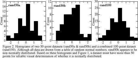
When we have 50 or 100 measurements instead of 20, we find that a finer histogram-binning interval is better for visualizing the pattern of the data. Figure 2 shows that an interval of about 0.5 is best for 100 measurements of this data type.

*     *     *

Normal Distribution

The data shown in Figures 1 and 2 have what is called a normal distribution. Such a distribution is formally called a Gaussian distribution or informally called a bell curve. The normal distribution has both a theoretical and an empirical basis. Theoretically, we expect a normal distribution whenever some parameter or variable X has many independent, random causes of variation and several of these so-called ‘sources of variance’ have effects of similar magnitude. Even if an individual type of error is non-normally distributed, groups of such errors are. Empirically, countless types of measurements in all scientific fields exhibit a normal distribution. Yet we must always verify the assumption that our data follow a normal distribution. Failure to test this assumption is scientists’ most frequent statistical pitfall. This mistake is needless, because one can readily examine a dataset to determine whether or not it is normally distributed.

Mean and Standard Deviation

For any dataset that follows a normal distribution, regardless of dataset size, virtually all of the information is captured by only three variables:

N: the number of data points, or measurements;
: the mean value; and
σ: the standard deviation.

The mean (), also called the arithmetic mean, is an average appropriate only for normal distributions. The mean is defined as:

or, in shortened notation, = Σx_i/N. The mean is simply the sum of all the individual measurement values, divided by the number of measurements.

The standard deviation (σ) is a measure of the dispersion or scatter of data. Defined as the square root of the variance (σ²), it is appropriate only for normal distributions. The variance is defined as:

σ² = Σ(x_i-)²/N.

Thus the variance is the average squared deviation from the mean, i.e., the sum of squared deviations from the mean divided by the number of data points. Computer programs usually avoid handling each measurement twice (first to calculate the mean and later to calculate the variance) by using an alternative equation: σ² = N^-1Σ(x_i²)-².

The standard deviation and variance are always positive. The units of standard deviation are the same as those of the x data. Often one needs to compare the scatter to the average value; two handy measures of this relationship are the fractional standard deviation (σ/) and percentage standard deviation (100σ/).

Normal Distribution Function

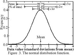
The normal distribution function, or ‘normal error function’, is shown in Figure 3. This probability distribution function of likely X values is expressed in terms of the ‘true mean’ M and standard deviation σ as:

f(x) = (1/σ(2π^0.5)e^{-(x-M)^2/2σ^2}.

For data drawn from a normal distribution, we can expect about 68.3% of the measurements to lie within one standard deviation of the mean, with half of the 68.3% above the mean and half below. Similarly, 95.4% of the measurements will lie within two standard deviations of the mean (i.e., within the interval -2σ < x_i < +2σ), and 99.7% of the measurements will lie within three standard deviations of the mean. These percentages are the areas under portions of the normal distribution function, as shown in Figure 3. All statistics books explain how to find the area under any desired portion of the curve, i.e., how to find the expected proportion of the data that will have values between specified limits. Of course, for the finite number of measurements of an individual dataset, we will only approximately observe these percentages. Nevertheless, it is well worth memorizing the following two approximations: two thirds of data lie within one standard deviation of the mean, and 95% lie within two standard deviations.

Although calculation of both the mean and standard deviation involves division by N, both are relatively independent of N. In other words, increasing the number of data points does not systematically increase or decrease either the mean or the standard deviation. Increasing the number of data points, however, does increase the usefulness of our calculated mean and standard deviation, because it increases the reliability of inferences drawn from them.

Based on visual examination of a histogram, it may be difficult to tell whether or not the data originate from a normally distributed parent population. For small N such as N=20 in Figure 1, random variations can cause substantial departures from the bell curve of Figure 3, and only the coarsest binning interval (Figure 1c) looks somewhat like a simple normal distribution. Even with N=50, the two samples in Figure 2 visually appear to be quite different, although both were drawn from the same table of random normal numbers. With N=100, the distribution begins to approximate closely the theoretical normal distribution (Figure 3) from which it was drawn. Fortunately, the mean and standard deviation are more robust; they are very similar for the samples of Figures 1 and 2.

The mean provides a much better estimate of the true value of X (the ‘true mean’ M) than do any of the individual measurements of X, because the mean averages out most of the random errors that cause differences between the individual measurements. How much better the mean is than the individual measurements depends on the dispersion (as represented by the standard deviation) and the number of measurements (N); more measurements and smaller standard deviation lead to greater accuracy of the calculated mean in estimating the true mean.

Our sample of N measurements is a subset of the parent population of potential measurements of X. We seek the value M of the parent population (the ‘true mean’). Finding the average of our set of measurements (the ‘calculated mean’) is merely a means to that end. We are least interested in the value x_i of any individual measurement, because it is affected strongly by unknown and extraneous sources of noise or scatter. If the data are normally distributed and unbiased, then the calculated mean is the most probable value of the true average of the parent population. Thus the mean is an extremely important quantity to calculate. Of course, if the data are biased such as would occur with a distorted yardstick, then our estimate of the true average is also biased. We will return later to the effects of a non-normal distribution.

Just as one can determine the mean and standard deviation of a set of N measurements, one can imagine undertaking several groups of N measurements and then calculating a grand mean and standard deviation of these groups. This grand mean would be closer to the true mean than most of the individual means would be, and the scatter of the several group means would be smaller than the scatter of the individual measurements. The standard deviation of the mean (), also called the standard error of the mean, is: =σ/N^0.5. Note that unlike a sample standard deviation, the standard deviation of the mean does decrease with increasing N. This standard deviation of the mean has three far-reaching but underutilized applications: weighted averages, confidence limits for the true mean, and determining how many measurements one should make.

Weighted Mean

A weighted mean is the best way to average data that have different precisions, if we know or can estimate those precisions. The weighted mean is calculated like an ordinary mean, except that we multiply each measurement by a weighting factor and divide the sum of these products not by N but by the sum of the weights, as follows:

= Σw_ix_i / Σw_i where w_i is the weighting factor of the ith measurement. If we use equal weights, then this equation reduces to the equation for the ordinary mean. Various techniques for weighting can be used. If each of the values to be averaged is itself a mean with an associated known variance, then the most theoretically satisfying procedure is to weight each value according to the inverse of the variance of the mean: w_i = 1/ = N/σ²_i. The weighted variance is:  = 1/Σ(1/) = 1/Σw_i.

For example, suppose that three laboratories measure a variable Y and obtain the following:

	N	mean	σ	(=σN-0.5)	wi
lab 1:	20	109	10	2.24	0.2
lab 2:	20	105	7	1.57	0.41
lab 3:	50	103	7	0.99	1.02

Then =(0.20•109 + 0.41•105 + 1.02•103)/(0.20+0.41+1.02) = 104.2. The variance of this weighted mean is  = 1/(0.20+0.41+1.02) = 0.613, and so the standard deviation of the weighted mean is  = 0.78. Note that the importance or weighting of the measurements from Lab 2 is twice as high as from Lab 1, entirely because Lab 2 was able to achieve a 30% lower standard deviation of measurements than Lab 1 could. Lab 3, which obtained the same standard deviation as Lab 2 but made 2.5 times as many measurements as Lab 2, has 2.5 times the importance or weighting of results.

95% Confidence Limits on Mean

Usually we want to use our measurements to make a quantitative estimate of the true mean M. One valuable way of doing so is to state the 95% confidence limits on the true mean, which for convenience we will call α₉₅. Confidence limits for the true mean M can be calculated as follows:

95% confidence limits:  α₉₅=•t₉₅   -α₉₅ < M < +α₉₅

99% confidence limits:  α₉₉=•t₉₉   -α₉₉ < M < +α₉₉

Just multiply the standard error of the mean by the ‘t-factor’, finding the t-factor in the table below for the appropriate number of measurements.

By stating the mean (our best estimate of the true mean M) and its 95% confidence, we are saying that there is only a 5% chance that the true mean is outside the range ±α₉₅. One’s desire to state results with as high a confidence level as possible is countered by the constraint that higher confidence levels encompass much broader ranges of potential data values. For example, our random-number dataset (N=100, =0.095, =0.02) allows us to state with 95% confidence that the true mean lies within the interval -0.17 to 0.21 (i.e., ± α₉₅, or 0.02 ± 0.19). We can state with 99% confidence that the true mean is within the interval -0.23 to 0.27. Actually the true mean for this dataset is zero.

Selection of a confidence level (α₉₅, α₉₉, etc.) usually depends on one’s evaluation of which risk is worse: the risk of incorrectly identifying a variable or effect as significant, or the risk of missing a real effect. Is the penalty for error as minor as having a subsequent researcher correct the error, or could it cause disaster such as an airplane crash? If prior knowledge suggests one outcome for an experiment, then rejection of that outcome needs a higher than ordinary confidence level. For example, no one would take seriously a claim that an experiment demonstrates test-tube cold fusion at the 95% confidence level; a much higher confidence level plus replication was demanded. Most experimenters use either a 95% or 99% confidence level. Tables for calculation of confidence limits other than 95% or 99%, called tables of the t distribution, can be found in any statistics book.

How Many Measurements are Needed?

The standard error of the mean is also the key to estimating how many measurements to make. The definition =σN^-0.5 can be recast as N=σ²/. Suppose we want to make enough measurements to obtain a final mean that is within 2 units of the true mean (i.e., ≤2), and a small pilot study permits us to calculate that our measurement scatter σ≈10. Then our experimental series will need N≥10²/2², or N≥25, measurements to obtain the desired accuracy at the 68% confidence level (or 1). For about 95% confidence, we recall that about 95% of points are within 2σ of the mean and conclude that we would need 2 ≤2, so N≥10²/1², or N≥100 measurements. Alternatively and more accurately, we can use the t table above to determine how many measurements will be needed to assure that our mean is within 2 units of the true mean at the 95% confidence level (α₉₅≤2): we need for t₉₅=α₉₅/ =α₉₅ N^0.5/σ= 2 N^0.5/10 = 0.2 N^0.5 to be greater than the t₉₅ in the table above for that N. By trying a few values of N, we see that N≥100 is needed.

As a rule of thumb, one must quadruple the number of measurements in order to double the precision of the result. This generalization is based on the N^0.5 relationship of standard deviation to standard error and is strictly true only if our measure of precision is the standard error. If, as is often the case, our measure of precision is α₉₅, then the rule of thumb is only approximately true because the t’s of Table 1 are only approximately equal to 2.0.

*     *     *

Propagation of Errors

Sometimes the variable of interest actually is calculated from measurements of one or more other variables. In such cases it is valuable to see how errors in the measured variables will propagate through the calculation and affect the final result. Propagation of errors is a scientific concern for several reasons:

• it permits us to calculate the uncertainty in our determination of the variable of interest;
• it shows us the origin of that uncertainty; and
• a quick analysis of propagation of errors often will tell us where to concentrate most of our limited time resources.

If several different independent errors (e_i) are responsible for the total error (E) of a measurement, then:

E² = e₁²+e₂²+… +e_N²

As a rule of thumb, one can ignore any random error that is less than a quarter the size of the dominant error. The squaring of errors causes the smaller errors to contribute trivially to the total error. If we can express errors in terms of standard deviations and if we have a known relationship between error-containing variables, then we can replace the estimate above with the much more powerful analysis of propagation of errors which follows.

Suppose that the variable of interest is V, and it is a function of the several variables a, b, c, …: V=f(a,b,c,…). If we know the variances of a, b, c, …, then the variance of V can be calculated from:

σ²_V = (∂V/∂a)²•σ²_a + (∂V/∂b)²•σ²_b +…    (1)

Thus the variance of V is equal to the sum of the product of each individual variance times the square of the partial derivative. For example, if we want to determine the area (A) of a rectangle by measuring its two sides (a and b): A=ab, and σ²_A = (∂A/∂a)²•σ²_a + (∂A/∂b)²•σ²_b = ²σ²_a + ²σ²_b. Propagation of errors can be useful even for single-variable problems. For example, if we want to determine the area (A) of a circle by measuring its radius (r): A=πr², and σ²_A = (∂A/∂r)²•σ²_r = (2π)²σ²_r.

Why analyze propagation of errors? In the example above of determining area of a circle from radius, we could ignore propagation of errors, just convert each radius measurement into an area, and then calculate the mean and standard deviation of these area determinations. Similarly, we could calculate rectangle areas from pairs of measurements of sides a and b, then calculate the mean and standard deviation of these area determinations. In contrast, each of the following variants on the rectangle example would benefit from analyzing propagation of errors:

• measurements a and b of the rectangle sides are not paired; shall we arbitrarily create pairs for calculation of A, or use propagation of errors?

• we have different numbers of measurements of rectangle sides a and b. We must either discard some measurements or, better, use propagation of errors;

• we are about to measure rectangle sides a and b and we know that a will be about 10 times as big as b. Because σ²_A = ²σ²_a + ²σ²_b, the second term will be about 100 times as important as the first term if a and b have similar standard deviations, and we can conclude that it is much more important to find a way to reduce σ²_b than to reduce σ²_a.

Usually we are less interested in the variance of V than in the variance of the mean V, or its square root (the standard error of V). We can simply replace the variances in equation (1) above with variances of means. Using variances of means, propagation of errors allows us to estimate how many measurements of each of the variables a,b,c,…  would be needed to determine V with some desired level of accuracy, if we have a rough idea of what the expected variances of a,b,c, … will be. Typically the variables a,b,c,…  will have different variances which we can roughly predict after a brief pilot study or before we even start the controlled measurement series. If so, a quick analysis of propagation of errors will suggest concentrating most of our limited time resources on one variable, either with a large number of measurements or with slower and more accurate measurements. For example, above we imagined that a is about 10 times as big as b and therefore concluded that we should focus on reducing σ²_b instead of reducing σ²_a. Even if we have no way of reducing σ²_b, we can reduce σ²(variance of mean b) by increasing the number of measurements, because the standard error =σN^-0.5.

Equation (1) and ability to calculate simple partial derivatives will allow one to analyze propagation of errors for most problems. Some problems are easier if equation (1) is recast in terms of fractional standard deviations:

(σ_v/V)² = (V^-1•∂V/∂a)²•σ²_a + (V^-1•∂V/∂b)²•σ²_b +…    (2)

Based on equation (1) or (2), here are the propagation of error equations for several common relationships of V to the variables a and b, where k and n are constants:

V=ka+nb:  σ²_v = k²σ²_a + n²σ²_b

V=ka-nb:   σ²_v = k²σ²_a + n²σ²_b

V=kab:      σ²_v = (kσ_a)² + (kσ_b)²

      or:      (σ_v/)² = (σ_a/)² + (σ_b/)²

V=ka/b:     (σ_v/)² = (σ_a/)² + (σ_b/)²

V=kaⁿ:       σ_v/ = nσ_a/

V=a^kbⁿ:     (σ_v/)² = (kσ_a/)² + (nσ_b/)²

*     *     *

Non-Normal Distributions

The most frequent statistics pitfall is also a readily avoided pitfall: assuming a normal distribution when the data are non-normally distributed. Every relationship and equation in the previous section should be used only if the data are normally distributed or at least approximately normally distributed. The more data depart from a normal distribution, the more likely it is that one will be misled by using what are called ‘parametric statistics’, i.e., statistics that assume a Gaussian distribution of errors. This section is organized in the same sequence that most data analyses should follow:

1) test the data for normality;
2) if non-normal, can one transform the data to make them normal?
3) if non-normal, should anomalous points be omitted?
4) if still non-normal, use non-parametric statistics.

Normality Tests

Because our statistical conclusions are often somewhat dependent on the assumption of a normal distribution, we would like to undertake a test that permits us to say “I am 95% confident that this distribution is normal.” But such a statement is no more possible than saying that we are 95% certain that a hypothesis is correct; disproof is more feasible and customary than proof. Thus our normality tests may allow us to say that “there is <5% chance that this distribution is normal” or, in statistical jargon,  “We reject the null hypothesis of a normal distribution at the 95% confidence level.”

Experienced scientists usually test data for normality subjectively, simply by looking at a histogram and deciding that the data look approximately normally distributed. Yet I, an experienced scientist, would not have correctly interpreted the center histogram of Figure 2 as from a normal distribution. If in doubt, one can apply statistical tests of normality such as Chi-square (χ²) and examine the type of departure from normality with measures such as skewness. Too often, however, even the initial subjective examination is skipped.

We can use a χ² test to determine whether or not our data distribution departs substantially from normality. A detailed discussion of the many applications of χ² tests is beyond the scope of this book, but almost all statistics books explain how a χ² test can be used to compare any data distribution to any theoretical distribution. A χ² test is most easily understood as a comparison of a data histogram with the theoretical Gaussian distribution. The theoretical distribution predicts how many of our measurements are expected to fall into each histogram bin. Of course, this expected frequency [Nf(n)] for the nth bin (or interval) will differ somewhat from the actual data frequency [F(n)], or number of values observed in that interval. Indeed, we saw in Figure 2 that two groups of 50 normally distributed measurements exhibited surprisingly large differences both from each other and from the Gaussian distribution curve. The key question then is how much of a difference between observed frequency and predicted frequency is chance likely to produce. The variable χ², which is a measure of the goodness of fit between data and theory, is the sum of squares of the fractional differences between expected and observed frequencies in all of the histogram bins:

Comparison of the value of χ² to a table of predicted values allows one to determine whether statistically significant non-normality has been detected. The table tells us the range of χ² values that are typically found for normal distributions. We do not expect values very close to zero, indicating a perfect match of data to theory. Nor do we expect χ² values that are extremely large, indicating a huge mismatch between the observed and predicted distributions.

The χ² test, like a histogram, can use any data units and almost any binning interval, with the same proviso that a fine binning interval is most appropriate when N is large. Yet some χ² tests are much easier than others, because of the need to calculate a predicted number of points for each interval. Here we will take the preliminary step of standardizing the data. Standardization transforms each measurement x_i into a unitless measurement which we will call z_i, where z_i = (x_i-)/σ. Standardized data have a mean of zero and a standard deviation of one, and any standardized array of approximately normally distributed data can be plotted on the same histogram. If we use a binning interval of 0.5σ, then the following table of areas under a normal distribution gives us the expected frequency [Nf(n)=N•area] in each interval.

Table 2: Areas of intervals of the normal distribution [Dixon and Massey, 1969].

σ Interval:	<-3	-3 to -2.5	-2.5 to -2	-2 to -1.5	-1.5 to -1	-1 to -0.5	-0.5 to 0.0
Area:	0.0013	0.0049	0.0166	0.044	0.0919	0.1498	0.1915
σ Interval:	>3	3 to 2.5	2.5 to 2	2 to 1.5	1.5 to 1	1 to 0.5	0.5 to 0.0

Equation 3 is applied to these 14 intervals, comparing the expected frequencies to the observed frequencies of the standardized data. Note that the intervals can be of unequal width. If the number of data points is small (e.g., N<20), one should reduce the 14 intervals (n=14) to 8 intervals by combining adjacent intervals of Table 2 [e.g., f(n) for 2σ to 3σ is .0166+.0049=.0215]. The following table shows the probabilities of obtaining a value of χ² larger than the indicated amounts, for n=14 or n=8. Most statistics books have much more extensive tables of χ² values for a variety of ‘degrees of freedom’ (df). When using such tables to compare a sample distribution to a Gaussian distribution that is estimated from the data rather than known independently, then df=n-2 as in Table 3.

Table 3. Maximum values of χ² that are expected from a normal distribution for different numbers of binning intervals (n) at various probability levels (P) [Fisher and Yates, 1963].

	P80	P90	P95	P97.5	P99	P99.5
n=8:	8.56	10.64	12.59	14.45	16.81	18.55
n=14:	15.81	18.55	21.03	23.34	26.22	28.3

For example, for n=14 intervals a χ² value of 22 (calculated from equation 3) would allow one to reject the hypothesis of a normal distribution at the 95% confidence level but not at 97.5% confidence (21.03<22<23.34).

 A non-normal value for χ² can result from a single histogram bin that has an immense difference between predicted and observed value; it can also result from a consistent pattern of relatively small differences between predicted and observed values. Thus the χ² test only determines whether, not how, the distribution may differ from a normal distribution.

Skewness is a measure of how symmetric the data distribution is about its mean. A distribution is positively skewed, or skewed to the right, if data extend substantially farther to the right of the peak than they do the left. Conversely, a distribution is negatively skewed, if data extend substantially farther to the left of the peak. A normal distribution is symmetric and has a skewness of zero. Later in this chapter we will see several examples of skewed distributions. A rule of thumb is that the distribution is reasonably symmetric if the skewness is between -0.5 and 0.5, and the distribution is highly skewed if the skewness is <-1 or >1.

*     *     *

If a data distribution is definitely non-normal, it might still be possible to transform the dataset into one that is normally distributed. Such a transformation is worthwhile, because it permits use of the parametric statistics above, and we shall soon see that parametric statistics are more efficient than non-parametric statistics. In some fields, transformations are so standard that the ordinary untransformed mean is called the arithmetic mean to distinguish it from means based on transformations.

The most pervasively suitable transformation is logarithmic: either take the natural logarithm of all measurements and then analyze them using techniques above, or simply calculate the geometric mean (): = Σ(x_i)^1/N. The geometric mean is appropriate for ratio data and data whose errors are a percentage of the average value. If data are positively skewed, it is worth taking their logarithms and redoing the histogram to see if they look more normal. More rarely, normality can be achieved by taking the inverse of each data point or by calculating a harmonic mean (): = N/Σ(1/x_i).

*     *     *

Rejecting Anomalous Data

Occasionally a dataset has one or more anomalous data points, and the researcher is faced with the difficult decision of rejecting anomalous data. In Chapter 6, we consider the potential pitfalls of rejecting anomalous data. In many scientists’ minds, data rejection is an ethical question: some routinely discard anomalous points without even mentioning this deletion in their publication, while others refuse to reject any point ever. Most scientists lie between these two extremes.

My own approach is the following:

• publish all data,
• flag points that I think are misleading or anomalous and explain why I think they are anomalous,
• show results either without the anomalous points or both with and without them, depending on how confident I am that they should be rejected.

In this way I allow the reader to decide whether rejection is justified, and the reader who may wish to analyze the data differently has all of the data available. Remembering that sometimes anomalies are the launching point for new insights, no scientist should hide omitted data from readers.

Here we will consider the question of data rejection statistically: are there statistical grounds for rejecting a data point? For example, if we have 20 measurements, we can expect about one measurement to differ from the mean by more than 2σ, but we expect (Table 2) that only 0.13% of the data points will lie more than three standard deviations below the mean. If one point out of 20 differs from the mean by more than 3σ, we can say that such an extreme value is highly unlikely to occur by chance as part of the same distribution function as the other data. Effectively, we are deciding that this anomalous point was affected by an unknown different variable. Can we conclude therefore that it should be rejected?

Although the entire subject of data rejection is controversial, an objective rejection criterion seems preferable to a subjective decision. One objective rejection criterion is Chauvenet’s criterion: a measurement can be rejected if the probability of obtaining it is less than 1/2N. For example, if N=20 then a measurement must be so distant from the mean that the probability of obtaining such a value is less than 1/40 or 2.5%. Table 4 gives these cutoffs, expressed as the ratio of the observed deviation (d_i) to the standard deviation, where the deviation from the mean is simply d_i = |x_i-|.

Table 4. Deviation from the mean required for exclusion of a data point according to Chauvenet’s criterion [Young, 1962].

N:	5	6	7	8	9	10	12	14	16	18	20
di/σ:	1.65	1.73	1.81	1.86	1.91	1.96	2.04	2.1	2.15	2.2	2.24
N:	25	30	40	50	60	80	100	150	200	400	1000
di/σ:	2.33	2.39	2.49	2.57	2.64	2.74	2.81	2.93	3.02	3.23	3.48

What mean and standard deviation should one use in applying Chauvenet’s criterion? The calculated mean and especially standard deviation are extremely sensitive to extreme points. Including the suspect point in the calculation of and σ substantially decreases the size of d_i/σ and thereby decreases the likelihood of rejecting the point. Excluding the suspect point in calculating the mean and standard deviation, however, is tantamount to assuming a priori what we are setting out to test; such a procedure often would allow us to reject extreme values that are legitimate parts of the sample population. Thus we must take the more conservative approach: the mean and standard deviation used in applying Chauvenet’s criterion should be those calculated including the suspect point.

If Chauvenet’s criterion suggests rejection of the point, then the final mean and standard deviation should be calculated excluding that point. In theory, one then could apply the criterion again, possibly reject another point, recalculate mean and standard deviation again, and continue until no more points can be rejected. In practice, this exclusion technique should be used sparingly, and applying it more than once to a single dataset is not recommended.

Often one waffles about whether or not to reject a data point even if rejection is permitted by Chauvenet’s criterion. Such doubts are warranted, for we shall see in later examples that Chauvenet’s criterion occasionally permits rejection of data that are independently known to be reliable. An alternative to data rejection is to use some of the nonparametric statistics of the next section, for they are much less sensitive than parametric techniques are to extreme values.

*     *     *

Median, Range, and 95% Confidence Limits

Until now, we have used parametric statistics, which assume a normal distribution. Nonparametric statistics, in contrast, make no assumption about the distribution. Most scientific studies employ parametric, not nonparametric, statistics, for one of four reasons:

• experimenter ignorance that parametric statistics should only be applied to normal distributions;
• lack of attention to whether or not one’s data are normally distributed;
• ignorance about nonparametric statistical techniques;
• greater efficiency of parametric statistics.

The first three reasons are inexcusable; only the last reason is scientifically valid. In statistics, as in any other field, assumptions decrease the scope of possibilities and enable one to draw conclusions with greater confidence, if the assumption is valid. For example, various nonparametric techniques require 5-50% more measurements than parametric techniques need to achieve the same level of confidence in conclusions. Thus nonparametric techniques are said to be less efficient than parametric techniques, and the latter are preferable if the assumption of a normal distribution is valid. If this assumption is invalid but made anyway, then parametric techniques not only overestimate the confidence of conclusions but also give somewhat biased estimates.

The nonparametric analogues of parametric techniques are:

Measure                Parametric                    Nonparametric
Average:                Mean                           Median
Dispersion:            Standard deviation       Interquartile range
Confidence limits: Conf. limits on mean   Conf. limits on median

Nonparametric statistics are easy to use, whether or not they are an option in one’s spreadsheet or graphics program. The first step in nearly all nonparametric techniques is to sort the measurements into increasing order. This step is a bit time consuming to do by hand for large datasets, but today most datasets are on the computer, and many software packages include a ‘sort’ command. We will use the symbol I_i to refer to the data value in sorted array position i; for example, I₁ would be the smallest data value.

The nonparametric measure of the true average value of the parent population is the median. For an odd number of measurements, the median is simply the middle measurement (I_N/2), i.e., that measurement for which half of the other measurements is larger and half is smaller. For an even number of measurements there is no single middle measurement, so the median is the average (midpoint) of the two measurements that bracket the middle. For example, if a sorted dataset of five points is 2.1, 2.1, 3.4, 3.6, and 4.7, then the median is 3.4; if a sorted dataset of six points is 2.1, 2.1, 3.4, 3.6, 4.7, and 5.2, then the median is (3.4+3.6)/2 = 3.5.

The median divides the data population at the 50% level: 50% are larger and 50% are smaller. One can also divide a ranked dataset into four equally sized groups, or quartiles. One quarter of the data are smaller than the first quartile, the median is the second quartile, and one quarter of the data are larger than the third quartile.

The range is a frequently used nonparametric measure of data dispersion. The range is the data pair of smallest (I₁) and largest (I_N) values. For example, the range of the latter dataset above is 2.1-5.2. The range is a very inefficient measure of data dispersion; one measurement can change it dramatically. A more robust measure of dispersion is the interquartile range, the difference between the third and first quartiles. The interquartile range ignores extreme values. It is conceptually analogous to the standard deviation: the interquartile range encompasses the central 50% of the data, and ±1 standard deviation encompasses the central 68% of a normal distribution,

For non-normal distributions, confidence limits for the median are the best way to express the reliability with which the true average of the parent population can be estimated. Confidence limits are determined by finding the positions I_k and I_N-k+1 in the sorted data array I_i, where k is determined from Table 5 below. Because these confidence limits use an integer number of array positions, they do not correspond exactly to 95% or 99% confidence limits. Therefore Table 5 gives the largest k yielding a probability of at least the desired probability. For example, suppose that we have 9 ranked measurements: 4.5, 4.6, 4.9, 4.9, 5.2, 5.4, 5.7, 5.8, and 6.2. Then N=9, k=3 yields less than 95% confidence, k=2 yields the 96.1% confidence limits 4.6-5.8, and k=1 yields 99.6% confidence limits 4.5-6.2.

Table 5. Confidence limits for the median [Nair, 1940; cited by Dixon and Massey, 1969].

N	k	α>95	k	α>99	N	k	α>95	k	α>99	N	k	α>95	k	α>99
6	1	96.9	-		26	8	97.1	7	99.1	46	16	97.4	14	99.5
7	1	98.1	-		27	8	98.1	7	99.4	47	17	96	15	99.2
8	1	99.2	1	99.2	28	9	96.4	7	99.6	48	17	97.1	15	99.4
9	2	96.1	1	99.6	29	9	97.6	8	99.2	49	18	95.6	16	99.1
10	2	97.9	1	99.8	30	10	95.7	8	99.5	50	18	96.7	16	99.3
11	2	98.8	1	99.9	31	10	97.1	8	99.7	51	19	95.1	16	99.5
12	3	96.1	2	99.4	32	10	98	9	99.3	52	19	96.4	17	99.2
13	3	97.8	2	99.7	33	11	96.5	9	99.5	53	19	97.3	17	99.5
14	3	98.7	2	99.8	34	11	97.6	10	99.1	54	20	96	18	99.1
15	4	96.5	3	99.3	35	12	95.9	10	99.4	55	20	97	18	99.4
16	4	97.9	3	99.6	36	12	97.1	10	99.6	56	21	95.6	18	99.5
17	5	95.1	3	99.8	37	13	95.3	11	99.2	57	21	96.7	19	99.2
18	5	96.9	4	99.2	38	13	96.6	11	99.5	58	22	95.2	19	99.5
19	5	98.1	4	99.6	39	13	97.6	12	99.1	59	22	96.4	20	99.1
20	6	95.9	4	99.7	40	14	96.2	12	99.4	60	22	97.3	20	99.4
21	6	97.3	5	99.3	41	14	97.2	12	99.6	61	23	96	21	99
22	6	98.3	5	99.6	42	15	95,6	13	99.2	62	23	97	21	99.3
23	7	96.5	5	99.7	43	15	96.8	13	99.5	63	24	95.7	21	99.5
24	7	97.7	6	99.3	44	16	95.1	14	99	64	24	96.7	22	99.2
25	8	95.7	6	99.6	45	16	96.4	14	99.3	65	25	95.4	22	99.4

Nonparametric statistics make no assumptions about the shape of either the parent population or the data distribution function. Thus nonparametric statistics cannot recognize that any data value is anomalous, and data rejection criteria such as Chauvenet’s criterion are impossible. In a sense, nonparametric statistics are intermediate between rejection of a suspect point and blind application of parametric statistics to the entire dataset; no points are rejected, but the extreme points receive much less weighting than they do when a normal distribution is assumed.

One fast qualitative (‘quick-and-dirty’) test of the suitability of parametric statistics for one’s dataset is to see how similar the mean and median are. If the difference between them is minor in comparison to the size of the standard deviation, then the mean is probably a reasonably good estimate, unbiased by either extreme data values or a strongly non-normal distribution. A rule of thumb might be to suspect non-normality or anomalous extreme values if 4(-X_m)>σ, where X_m is the median.

*     *     *

Figure 4. Flowchart of decision steps for a group of measurements.

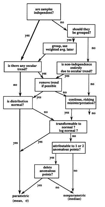
Figure 4 is a flowchart that shows one possible way of approaching analysis of a variable. Rarely does anyone evaluate a variable as systematically as is shown in Figure 4; indeed, I have never seen such a flowchart or list of steps. This flowchart demonstrates why different examples, such as those in the following section, require different treatments.

A useful first step in analyzing a variable is to ask oneself whether the individual observations, measurements, or data are independent. Two events are independent if they are no more likely to be similar than any two randomly selected members of the population. Independence is implicit in the idea of random errors; with random errors we expect that adjacent measurements in our dataset will be no more similar to each other than distant measurements (e.g., first and last measurements) will be. Independence is an often-violated assumption of the single-variable statistical techniques. Relaxation of this assumption sometimes is necessary and permissible, as long as we are aware of the possible complications introduced by this violation (note that most scientists would accept this statement pragmatically, although to a statistician this statement is as absurd as saying A≠A). Except for the random-number example, none of the example datasets to follow has truly independent samples. We will see that lack of independence is more obvious for some datasets than for others, both in a priori expectation and in data analysis.

Actual scientific data have the same problem: sometimes we expect our measurements to be unavoidably non-independent, whereas at other times we expect independence but our analysis reveals non-independence. Thus, regardless of expectations, one should plot every dataset as a function of measurement sequence, for visual detection of any unexpected secular trends. Examination of the data table itself often is an inadequate substitute. No statistical test detects secular trends as consistently as simple examination of a plot of variable vs. measurement order. Examples of such unexpected secular trends are:

• instrumental drift;
• measurement error during part of the data acquisition;
• undetected, involuntary change of part of the measurement procedure during the measurement series;
• undetected change in standards;
• temporal change in an unidentified relevant variable, i.e., a source of ‘noise’.

*     *     *

Examples

We can gain insight into the statistical techniques described above by considering their application to a few datasets of different types. Our examples come from a variety of original sources, but I got almost all of them from the World Almanac [Hoffman, 1990]. The exceptions are the examples of random normal numbers and of the hare and tortoise. I have deliberately chosen familiar examples rather than artificial data or real scientific data, because the explanation for observed statistical behavior is easier to comprehend with familiar examples. The examples are:

• reexamination of the random normal numbers of Figures 1 and 2;
• race between the hare and the tortoise;
• percentage of high school students that graduate, by state;
• state population (1990 census);
• state taxes, per capita, by state;

Table 6 summarizes the statistical results for these examples, as well as some examples introduced in the next chapter.

Table 6. Summary statistics for the example problems used in this chapter and in Chapter 3. Statistics for population, taxes, and batting averages are shown both before and after exclusion of extreme points. Columns 2-7: parametric; columns 8-10: nonparametric; column 11: exclusion by Chauvenet’s criterion (Y or N).

dataset	N		σ	α95	skew		med.	range	α95	Ch?
rand100	100	0.02	0.95	0.19	-0.1	0.1	0.11	-2.4/2.2	-0.28/0.39	N
rand50a	50	0.05	0.98	0.28	-0.4	0.14	0.16	-2.4/1.9	-0.28/0.39	N
rand50b	50	-0.01	0.94	0.27	0.1	0.13	0.03	-1.9/2.2	-0.4/0.4	N
rand20a	20	0.03	0.9	0.42	-1	0.2	0.19	-2.4/1.3	-0.11/0.39	Y
rand20b	20	0.39	0.95	0.42	-0.1	0.21	0.53	-0.9/1.9	-0.55/1.23	N
pop	50	4.9	5.38	1.53	2.4	0.76	3.34	.4/29.3	2.3/4.8	Y
pop -1	49	4.41	4.11	1.18	1.5	0.59	3.27	.4/17.6	2.3/4.7	Y
ln(pop)	50	1.11	1.01	0.29	0	0.14	1.21	-0.8/3.4	0.8/1.6	N
taxes	50	1140	343	97	2	48	1056	553/2674	993/1161	Y
tax -1	49	1109	265	76	0.8	38	1055	553/1993	993/1141	Y
deficit	30	10.6	7.5	2.8	0.2	1.4	11.3	-1.8/25.7	5.5/14.1	N
HS grad	50	75.1	7.4	2.1	-0.1	1.1	76.2	58/90	72.9/78.0	N
smoked	10	69.6	31.2	22.3	0.5	9.8	69.2	65.7/75.3	66.4/73.6	N
Anch T	12	35.2	16.8	10.7	0	4.9	35	13/58	18/54	N
bat avg	90	352	21	4.5	0.9	2.3	350	313/424	342/354	Y
bat -30	60	347	15	3.9	0.2	1.9	346	313/385	341/353	N

Example 1: random normal numbers of Figures 1 and 2.

The data of Figures 1 and 2 are drawn from a table of random normal numbers and therefore are about as close as one can get to perfectly random, normally distributed data. The true population mean is zero, and the true population standard deviation is one; data units therefore could be called ‘true standard deviations’. We will consider five datasets: one with N=100 (Rand100), two with N=50 (Rand50a & Rand50b), and two with N=20 (Rand20a & Rand20b). Measurements within each dataset are independent of each other, but datasets are not strictly independent: the N=100 example is the combination of the two N=50 examples, and the two N=20 examples are included in the first N=50 example.

All five examples have a mean (Table 6) that is very close to the true population mean of zero; the largest departure is 0.4 units. As we might expect, the calculated 95% confidence limits for the true mean (α₉₅) include zero for all five examples. The α₉₅ for Rand20b, however, barely includes the true mean of zero. At first it seems surprising that we have almost disproved something that we know to be true: that the true mean is zero. We should remember, however, that if we did this test on 20 datasets instead of 5, we would expect an average of one test to ‘fail’ at the 95% confidence level.

The histograms of Figure 2 show considerable apparent character change when compared either to each other or to a theoretical normal distribution. This variability is typical sampling variability for small samples. This visual variability is mirrored by a variability in calculated skewness: one of the five (Rand20a) actually fails the rule of thumb that skewness should be less than ±0.5 for normally distributed data. In spite of the apparently substantial departures from a simple normal distribution in the histograms, the standard deviation is fairly robust: the standard deviation of each is about the same (0.90-0.98) and close to the true population value of 1.0. By coincidence, all five standard deviations are less than the true value of 1.0; such a coincidence would be highly unlikely (1 chance in 25) if the five datasets were truly independent rather than subsets of each other. The interquartile range, which is less efficient than the standard deviation, is similar (1.32-1.47) for the three larger datasets but highly variable (0.62-1.86) for the 20-point samples.

Rand20a, the apparently skewed dataset, is also the only dataset for which Chauvenet’s criterion allows us to reject a measurement as anomalous. This same measurement of -2.41 was in Rand100 and Rand50a, but it was not considered rejectable by application of Chauvenet’s criterion to those two datasets because more extreme values are expected when N is larger. Obviously (in hindsight), even exceedingly scarce extreme values will occasionally show up in small samples, seeming more anomalous in the small sample than in a large sample. Chauvenet’s criterion was incorrect in suggesting that the measurement be rejected from Rand20a.

In all five examples, the median lies farther from the true mean of zero than the arithmetic mean does. Thus for these samples from a normally distributed parent population, the median is a less efficient and therefore less accurate estimate of the true population average than is the mean. Similarly, the range varies substantially among the different examples, though we have seen that the standard deviation is relatively constant. For each of the five examples, the 95% confidence limits for the median are broader and therefore less efficient that 95% confidence limits for the mean; in every case these confidence limits for the median correctly includes the true population average of zero. Whether we use confidence limits for the mean or for the median, we see in Table 6 that making 100 measurements rather than 20 lets us narrow our uncertainties in estimating the true population average by 50% or more.

Example 2: race between the hare and the tortoise.

In an update of the ancient race between the hare and the tortoise, the tortoise won the race and yet the hare got a speeding ticket. Since the tortoise won, its ‘average’ speed must have been faster than the hare’s more erratic pace. Use of a mean and standard deviation would be quite inappropriate for the hare. The hare had a bimodal speed of either zero (resting) or -- rarely -- extremely fast; probably the mean would be closer to the dominant zero peak and the standard deviation would imply some negative speeds. Sampling the hare’s speed at uniform time intervals would give a completely different picture than if its speed were sampled at uniform distance intervals: according to the former it was usually resting, but according to the latter it was usually breaking the speed limit.

Example 3: percentage of high school students that graduate, by state.

We cannot expect values of any variable for different states of the U.S.A. to be truly independent: adjacent states or states with similar industries could be expected to give more similar values than distant states with different economic bases. We will proceed anyway, because such examples are illustrative and because it is fruitless to respond to a question like “What is the average percentage of students that graduate from U.S. high schools?” with the answer “It is impossible to say, because it is invalid to average such data.”

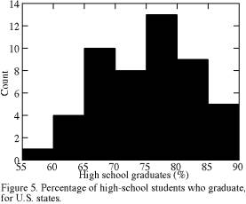
Figure 5 shows that the distribution of high-school graduation rates appears to be approximately normal. Indeed, it looks more like a bell-shaped or Gaussian distribution than do Figures 1 and 2 (which are known to come from a normally distributed parent population). Furthermore, skewness is low, and Chauvenet’s criterion does not reject any data. Thus it is relatively safe to conclude that the calculated average graduation percentage is 75.1% and that the ‘true’ average is 75.1±2.1%. Nonparametric statistics are neither needed nor as appropriate as parametric statistics for this dataset. The mean value of 75.1 is close to the median of 76.2, at least in comparison to the high standard deviation of 7.4, again suggesting normality.

Example 4: population of U.S. states (1990 census).

The populations, in millions, of the U.S. states obviously diverge from a normal distribution (Figure 6a). Our ‘quick-and-dirty’ technique of comparing mean to median indicates a non-normal distribution: the mean is almost 50% larger than the median, and examination of Figure 6a suggests that one anomalously high value is at least partially responsible for pulling the mean so far to the right of the median. The distribution has a strong positive skewness of 2.4, with no left tail and a long right tail.

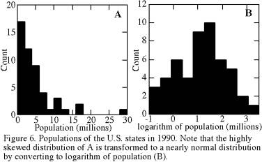
Should the one extremely large value of 29,279,000 (29.3 million or 29.3M) for California population be excluded as anomalous? Chauvenet’s criterion says that any value of >18.7M can be excluded, so 29.3M is far beyond the minimum cutoff. If we exclude California and recalculate mean and standard deviation, reapplication of Chauvenet’s criterion (not recommended) would suggest that we reject two more states with large populations. I have not done so, though it might be interesting to see how many states we would ultimately exclude through repeated use of Chauvenet’s criterion.

If one is statistically justified in excluding at least California, then such an exclusion implies that California is in some way unique or anomalous, with some different variable controlling its population than is operant (or at least important) for populations of the other states. As a former member of the California population, I can think of many ways in which one would describe the California population as anomalous, but that question is beyond the scopes of these data and of our concern. The key point is that the analysis flags an anomaly; it cannot explain the anomaly.

Figure 4 suggests that one’s first reaction to a non-normal distribution should not be to discard data; it is to consider transforms that might convert the dataset to an approximately normal distribution. The most common transform is to take natural logarithms of the data, and the logarithmic transform is most likely to succeed in cases such as the present one that have a strong positive skewness. Figure 6b is such a transform. Logarithm of population visually does appear to be normally distributed, mean and median are similar (with a difference that is only about 10% of the standard deviation), and skewness is zero (!). Thus we may conclude that state population is log-normally distributed, with a mean of 3.0M (e^1.1, because the mean of the natural logarithms of population is 1.1).

Knowing that it is much more appropriate to analyze logarithms of state populations than raw state populations, we can now apply Chauvenet’s test and find that no data should be excluded. Our previous temptation to exclude California was ill founded. With any logarithmic distribution the largest values tend to be more widely spaced than the smallest values. I suspect that Chauvenet’s criterion will recommend exclusion of one or even many valid data points whenever a dataset has strong skewness (positive or negative), because Chauvenet’s criterion is excessively sensitive to such violations of normality.

Example 5: average state taxes per capita, by state.

What is the average amount of state taxes paid in the U.S.? One answer might come from simply dividing the total of all state tax income by the total U.S. population. Here is another, more informative approach.

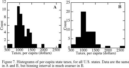
Histograms of state taxes per capita, by state, are shown in Figures 7a and 7b. Although the two histograms show the same data, they emphasize slightly different features because of their different binning intervals. The coarser binning interval of Figure 7b makes the distribution look more normal, as is often the case for coarser binning (within reason). Finer binning (Figure 7a) makes the largest datum, per capita taxes of $2674 ($2.7K) in Alaska, look more anomalous. Both histograms are roughly bell-shaped but positively skewed (skewness=2.0). Thus it is worth trying a transform to logarithm of per capita taxes, but such a distribution is not shown because it accomplishes no improvement.

Chauvenet’s criterion shows that the value for Alaska taxes is far more than is likely by chance for a normal distribution. Recalculation of parametric statistics after omitting Alaska gives a more normal value of skewness, and permits us to exclude yet another state (Hawaii), but we will forgo that opportunity. It seems likely that Alaska and possible that Hawaii are anomalous in state taxes in comparison to other states, because costs are greater at remote locations.