Chapter 3: Induction & Pattern Recognition
|
|
Induction is pattern recognition -- an inference based on limited observational or experimental data -- and pattern recognition is an addictively exhilarating acquired skill.
Of the two types of scientific inference, induction is far more pervasive and useful than deduction (Chapter 4). Induction usually infers some pattern among a set of observations and then attributes that pattern to an entire population. Almost all hypothesis formation is based consciously or subconsciously on induction.
Induction is pervasive because people seek order insatiably, yet they lack the opportunity of basing that search on observation of the entire population. Instead they make a few observations and generalize.
Induction is not just a description of observations; it is always a leap beyond the data -- a leap based on circumstantial evidence. The leap may be an inference that other observations would exhibit the same phenomena already seen in the study sample, or it may be some type of explanation or conceptual understanding of the observations; often it is both. Because induction is always a leap beyond the data, it can never be proved. If further observations are consistent with the induction, then they confirm, or lend substantiating support to, the induction. But the possibility always remains that as-yet-unexamined data might disprove the induction.
In symbols, we can think of confirmation of our inductive hypothesis A as: A⇒B, B, ∴A (i.e., A implies B; B is observed and therefore A must also be true or present). Such evidence may be inductively useful confirmation. The logic, however, is a deductive fallacy (known as affirming the consequent), because there may always be other factors that cause B. Although confirmation of an induction is incremental and inconclusive, the hypothesis can be disproved by a single experiment, via the deductive technique of modus tollens: A⇒B, -B, ∴-A (i.e., A implies B; B is not observed and therefore A must not be true or present).
Scientific induction requires that we make two unprovable assumptions, or postulates:
• representative sampling. Only if our samples are representative, or similar in behavior to the population as a whole, may we generalize from observations of these samples to the likely behavior of the entire population. In contrast, if our samples represent only a distinctive subset of the population, then our inductions cannot extend beyond this subset. This postulate is crucial, it is usually achieved easily by the scientist, and yet it is often violated with scientifically catastrophic results. As discussed more fully in the previous chapter, randomization and objective sampling are the paths to obtaining a representative sample; subjective sampling generates a biased sample.
• uniformity of nature. Strictly speaking, even if our sample is representative we cannot be certain that the unsampled remainder of the population exhibits the same behavior. However, we assume that nature is uniform, that the unsampled remainder is similar in behavior to our samples, that today’s natural laws will still be valid tomorrow. Without this assumption, all is chaos.
* * *
Induction is explanation, and explanation is identification of some type of order in the universe. Explanation is an integral part of the goal of science: perceiving a connection among events, deciphering the explanation for that connection, and using these inductions for prediction of other events. Some scientists claim that science cannot explain; it can only describe. That claim only pertains, however, to Aristotelian explanation: answering the question “Why?” by identifying the purpose of a phenomenon. More often, the scientific question is “How?” Here we use the inclusive concept of explanation as any identification of order.
Individual events are complex, but explanation discerns their underlying simplicity of relationships. In this section we will consider briefly two types of scientific explanation: comparison (analogy and symmetry) and classification. In subsequent sections we will examine, in much more detail, two more powerful types of explanation: correlation and causality.
Explanation can deal with attributes or with variables. An attribute is binary: either present or absent. Explanation of attributes often involves consideration of associations of the attribute with certain phenomena or circumstances. A variable, in contrast, is not merely present or absent; it is a characteristic whose changes can be quantitatively measured. Explanations of a variable often involve description of a correlation between changes in that variable and changes in another variable. If a subjective attribute, such as tall or short, can be transformed into a variable, such as height, explanatory value increases.
The different kinds of explanation contrast in explanatory power and experimental ease. Easiest to test is the null hypothesis that two variables are completely unrelated. Statistical rejection of the null hypothesis can demonstrate the likelihood that a classification or correlation has predictive value. Causality goes deeper, establishing the origin of that predictive ability, but demonstration of causality can be very challenging. Beyond causality, the underlying quantitative theoretical mechanism sometimes can be discerned.
* * *
Comparison is the most common means of identifying order, whether by scientists or by lay people. Often, comparison goes no farther than a consideration of the same characteristic in two individuals. Scientific comparison, however, is usually meant as a generalization of the behavior of variables or attributes. Two common types of comparison are symmetry and analogy.
Symmetry is a regularity of shape or arrangement of parts within a whole -- for example, a correspondence of part and counterpart. In many branches of science, recognition of symmetry is a useful form of pattern recognition. To the physicist, symmetry is both a predictive tool and a standard by which theories are judged.
In his book on symmetry, physicist Hermann Weyl [1952] said: “Symmetry, as wide or as narrow as you may define its meaning, is one idea by which man through the ages has tried to comprehend and create order, beauty, and perfection.”
I’ve always been confident that the universe’s expansion would be followed by a contraction. Symmetry demands it: big bang, expanding universe, gravitational deceleration, contracting universe, big crunch, big bang, … No problem of what happens before the big bang or after the big crunch; an infinite cycle in both directions. The only concern was that not enough matter had been found to generate sufficient gravity to halt the expansion. But dark matter is elusive, and I was sure that it would be found. Now, however, this elegant model is apparently overthrown by evidence that the expansion is accelerating, not decelerating [Schwarzschild, 2001]. Symmetry and simplicity do not always triumph.
Analogy is the description of observed behavior in one class of phenomena and the inference that this description is somehow relevant to a different class of phenomena. Analogy does not necessarily imply that the two classes obey the same laws or function in exactly the same way. Analogy often is an apparent order or similarity that serves only as a visualization aid. That purpose is sufficient justification, and the analogy may inspire fruitful follow-up research. In other cases, analogy can reflect a more fundamental physical link between behaviors of the two classes. Either type of analogy can bridge tremendous differences in size or time scale. For example, the atom and the solar system are at two size extremes and yet their orbital geometries are analogous from the standpoints of both visualization and Newtonian physics. Fractals, in contrast, also describe similar physical phenomena of very different sizes, but they go beyond analogy by genetically linking different scales into a single class.
Analogy is never a final explanation; rather it is a potential stepping-stone to greater insight and hypothesis generation. Unfortunately, however, analogy sometimes is misused and treated like firm evidence. The following two examples illustrate the power of exact analogy and the fallacy of remote analogy.
Annie Dillard [1974] on the analogy between chlorophyll and hemoglobin, the bases of plant and animal energy handling: “All the green in the planted world consists of these whole, rounded chloroplasts wending their ways in water. If you analyze a molecule of chlorophyll itself, what you get is one hundred thirty-six atoms of hydrogen, carbon, oxygen, and nitrogen arranged in an exact and complex relationship around a central ring. At the ring’s center is a single atom of magnesium. Now: If you remove the atom of magnesium and in its exact place put an atom of iron, you get a molecule of hemoglobin.”
Astronomer Francesco Sizi’s early 17th century refutation of Galileo’s claim that he had discovered satellites of Jupiter [Holton and Roller, 1958]:
“There are seven windows in the head, two nostrils, two ears, two eyes and a mouth; so in the heavens there are two favorable stars, two unpropitious, two luminaries, and Mercury alone undecided and indifferent. From which and many similar phenomena of nature such as the seven metals, etc., which it were tedious to enumerate, we gather that the number of planets is necessarily seven.”
Comparison often leads to a more detailed explanation: classification. Classification can extract simple patterns from a mind-numbing quantity of individual observations, and it is also a foundation for most other types of scientific explanation. Classification is the identification of grounds for grouping complexly divergent individuals into a single class, based on commonality of some significant characteristic. Every individual is different, but we need and value tools for coping with this diversity by identifying classes of attributes. Indeed, many neurobiologists have concluded that people never experience directly the uniqueness of individual objects; instead, we unconsciously fit a suite of schemata, or classifications, to our perceptions of each object (Chapter 6).
A class is defined arbitrarily, by identifying a minimal number of characteristics required for inclusion in the class. Recognizing a scientifically useful classification, however, requires inductive insight. Ideally, only one or a few criteria specify a class, but members of the class also share many other attributes. For example, one accomplishes little by classifying dogs according to whether or not they have a scar on their ear. In contrast, classifying dogs as alive or dead (e.g., based on presence/absence of heartbeat) permits a wealth of generally successful predictions about individual dogs. Much insight can be gained by examining these ancillary characteristics. These aspects need not be universal among the class to be informative. It is sufficient that the classification, although based on different criteria, enhances our ability to predict occurrence of these typical features.
Classes are subjectively chosen, but they are defined according to objective criteria. If the criteria involve presence or absence of an attribute (e.g., use of chlorophyll), definition is usually straightforward. If the criteria involve a variable, however, the definition is more obviously subjective in its specification of position (or range of positions) along a continuum of potential values.
A classification scheme can be counterproductive [Oliver, 1991], if it imposes a perspective on the data that limits our perception. A useful classification can become counterproductive, when new data are shoved into it even though they don’t fit.
Classifications evolve to regain utility, when exceptions and anomalous examples are found. Often these exceptions can be explained by a more restrictive and complex class definition. Frequently, the smaller class exhibits greater commonality of other characteristics than was observed within the larger class. For example, to some early astronomers all celestial objects were stars. Those who subdivided this class into ‘wandering stars’ (planets and comets) and ‘fixed stars’ would have been shocked at the immense variety that later generations would discover within these classes.
Each scientist applies personal standards in evaluating the scope and size of a classification. The ‘splitters’ favor subdivision into small subclasses, to achieve more accurate predictive ability. The ‘lumpers’ prefer generalizations that encompass a large portion of the population with reasonable but not perfect predictive accuracy. In every field of science, battles between lumpers and splitters are waged. For many years the splitters dominate a field, creating finer and finer classifications of every variant that is found. Then for a while the lumpers convince the community that the pendulum has swung too far and that much larger classes, though imperfect, are more worthwhile.
A class can even be useful though it has no members whatsoever. An ideal class exhibits behavior that is physically simple and therefore amenable to mathematical modeling. Even if actual individual objects fail to match exactly the defining characteristics of the ideal class, they may be similar enough for the mathematical relationships to apply. Wilson [1952] gives several familiar examples of an ideal class: physicists often model rigid bodies, frictionless surfaces, and incompressible fluids, and chemists employ the concepts of ideal gases, pure compounds, and adiabatic processes.
* * *
Classifications, like all explanations, seek meaningful associations and correlations. Sometimes, however, they are misled by coincidence.
“A large number of incorrect conclusions are drawn because the possibility of chance occurrences is not fully considered. This usually arises through lack of proper controls and insufficient repetitions. There is the story of the research worker in nutrition who had published a rather surprising conclusion concerning rats. A visitor asked him if he could see more of the evidence. The researcher replied, ‘Sure, there’s the rat.’” [Wilson, 1952]
Without attention to statistical evidence and confirmatory power, the scientist falls into the most common pitfall of non-scientists: hasty generalization. One or a few chance associations between two attributes or variables are mistakenly inferred to represent a causal relationship. Hasty generalization is responsible for many popular superstitions, but even scientists such as Aristotle were not immune to it. Hasty generalizations are often inspired by coincidence, the unexpected and improbable association between two or more events. After compiling and analyzing thousands of coincidences, Diaconis and Mostelle [1989] found that coincidences could be grouped into three classes:
• cases where there was an unnoticed causal relationship,
so the association actually was not a coincidence;
• nonrepresentative samples, focusing on one association while ignoring
or forgetting examples of non-matches;
• actual chance events that are much more likely than one might expect.
An example of this third type is that any group of 23 people has a 50% chance of at least two people having the same birthday.
Coincidence is important in science, because it initiates a search for causal relationships and may lead to discovery. An apparent coincidence is a perfectly valid source for hypotheses. Coincidence is not, however, a hypothesis test; quantitative tests must follow.
The statistical methods seek to indicate quantitatively which apparent connections between variables are real and which are coincidental. Uncertainty is implicit in most measurements and hypothesis tests, but consideration of probabilities allows us to make decisions that appropriately weigh the impact of the uncertainties. With suitable experimental design, statistical methods are able to deal effectively with very complex and poorly understood phenomena, extracting the most fundamental correlations.
* * *
“Every scientific problem is a search for the relationship between variables.” [Thurstone, 1925]
Begin with two variables, which we will call X and Y, for which we have several measurements. By convention, X is called the independent variable and Y is the dependent variable. Perhaps X causes Y, so that the value of Y is truly dependent on the value of X. Such a condition would be convenient, but all we really require is the possibility that a knowledge of the value of the independent variable X may give us some ability to predict the value of Y.
* * *
To introduce some of the concerns implicit in correlation
and pattern recognition, let’s begin with three examples: National League
batting averages, the government deficit, and temperature variations in Anchorage,
AK.
Example 1: highest annual batting average in the National League.
|
|
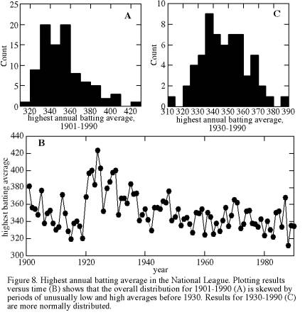
We consider here the maximum batting average obtained by any National League player in each of the years 1901-1990. Because batting average is a time series, data certainly are not independent and we must beware of temporal trends. If we were to ignore the possibility of temporal trends, we would conclude that the data exhibit moderately normal behavior (Figure 8a), with slight positive skewness and, according to Chauvenet’s criterion, one anomalously high value of 424 that could be excluded. Ignoring temporal trends, we would predict at a 68% confidence level (1σ) that the maximum 1991 batting average would be 352±21 (Table 6).
Plotting batting average versus time (Figure 8b), however, we see immediately that the departures from the mean were nonrandom. Batting averages decreased rapidly during 1901-1919, peaked during 1921-1930, and decreased gradually since then. What accounts for these long-term trends? I am not enough of a baseball buff to know, but I note that the 1921-1930 peak is dominated by Rogers Hornsby, who had the highest average in 7 of these 10 years. Often in such analyses, identification of a trend’s existence is the first step toward understanding it and, in some cases, toward preventing it.
Of course, substantial ‘noise’, or annual variation, is superimposed on these long-term trends. Later in this section, we will consider removal of such trends, but here we will take a simpler and less satisfactory approach: we will limit our data analysis to the time interval 1931-1990. We thereby omit the time intervals in which secular (temporal) trends were dominant. If this shorter interval still contains a slight long-term trend, that trend is probably too subtle to jeopardize our conclusions.
For 1931-1990 batting averages (Figure 8c), skewness is substantially less than for the larger dataset, and no points are flagged for rejection by Chauvenet’s criterion. The standard deviation is reduced by one third, but the 95% confidence limits are only slightly reduced because the decrease in number of points counteracts the improvement in standard deviation.
Confining one’s analysis to a subsample of the entire
dataset is a legitimate procedure, if one has objective grounds for defining the subset and
if one does not apply subset-based interpretations to the overall population.
Obviously it would be invalid to analyze a ‘subset’ such as batting
averages less than 400. Will the 1991 maximum batting average be 347±15 as
predicted by the 1931-1990 data, or will there be another Rogers Hornsby?
Example 2: U.S. government deficit as a percentage of outlays, for 1960-1989.
|
|
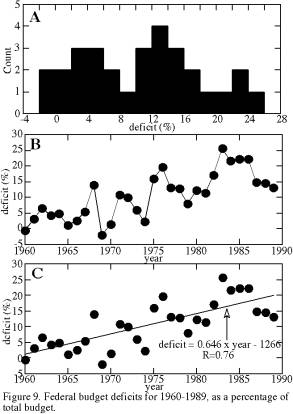
Again we are dealing with a time series, so the flowchart of Figure 4 recommends that our first step is to plot deficit percentage versus time (Figure 9b). Such a plot exhibits a strong secular trend of increasing deficit percentage, on which is superposed more ‘random’ year-to-year variations. In other words, the major source of variance in deficits is the gradual trend of increasing deficit, and annual variations are a subsidiary effect. Because our data are equally spaced in time, the superposition of these two variances gives a blocky, boxcar-like appearance to the histogram (Figure 9a), with too little tail. If the secular trend were removed, residuals would exhibit a more bell-shaped distribution.
If we ignore the secular trend, nonparametric statistics are more appropriate for this dataset than are parametric statistics. However, ignoring the major source of variance in a dataset is almost always indefensible. Instead, a secular trend can be quantified and used to refine our understanding of a dataset. Later in this chapter, we will return to this example and determine that secular trend.
Example 3: Monthly averages of temperature for Anchorage, Alaska.
|
|
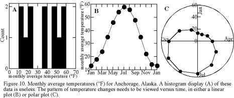
The histogram of monthly temperatures in Anchorage (Figure 10a) is strongly bimodal, with equal-sized peaks at 10-25° and at 45-60°. Skewness is zero because the two peaks are equal in size, so the mean is close to the median and both are a good estimate of the true average. Many bimodal distributions have one dominant peak, however, causing a distribution that is skewed and biasing both the mean and median.
Nonparametric statistics are much more appropriate here than parametric statistics. Neither is an acceptable substitute for investigation of the causes of a bimodal distribution. For this example, the answer lies in the temporal trends. Again we have a time series, so a plot of temperature versus time may lend insight into data variability. Months of a year can define an ‘ordinal’ scale: order along a continuum is known but there is neither a time zero nor implicitly fixed values. Here I simply assigned the numbers 1-13 to the months January-December-January for plotting, keeping in mind that the sequence wraps around so that January is both 1 and 13, then I replaced the number labels with month names (Figure 10b). A circular plot type known as polar coordinates is more appropriate because it incorporates wraparound (Figure 10c).
Consider the absurdities of simply applying parametric statistics to datasets like this one. We calculate that the average temperature is 35.2° (i.e., cold), but in fact the temperature almost never is cold. It switches rapidly from cool summer temperatures to bitterly cold winter temperatures. Considering just the standard deviation, we would say that temperature variation in Anchorage is like that in Grand Junction, Colorado (16.8° versus 18.7°). Considering just the mean temperature, we would say that the average temperature of Grand Junction (52.8°) is similar to that of San Francisco (56.8°). Thus temperatures in Grand Junction, Colorado are statistically similar to those of San Francisco and Anchorage!
* * *
Crossplots are the best way to look for a relationship between two variables. They involve minimal assumptions: just that one’s measurements are reliable and paired (xi, yi). They permit use of an extremely efficient and robust tool for pattern recognition: the eye. Such pattern recognition and its associated brainstorming are a joy.
Crossplot interpretation, like any subjective pattern recognition, is subject to the ‘Rorschach effect’: the brain's bias toward ‘seeing’ patterns even in random data. The primary defense against the Rorschach effect is to subject each apparent pattern to some quantitative test, but this may be impractical. Another defense is to look at many patterns, of both random and systematic origins, in order to improve one’s ability to distinguish between the two.
Galison [1985] described the application of this approach in the bubble-chamber experiments at Berkeley. A computer program plotted histograms not only of the measured data but also of randomly generated pseudo-datasets. The investigator had to distinguish his datasets by recognizing which histograms had significant peaks. Louis Alvarez said that this program prevented many mistaken discovery claims and later retractions. Figure 2 makes me empathize with the problem faced by these particle physicists.
|
|
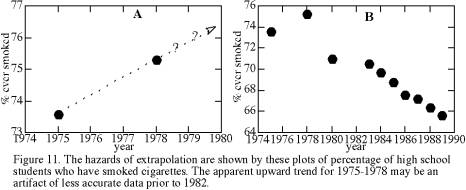
Data dispersion is inevitable with crossplots, and awareness of this dispersion is essential to crossplot interpretation. For example, consider the change through time of the percentage of American high school seniors who have ever smoked a cigarette. Figure 11a shows that this percentage increased from 73.6% to 75.3% in the three years from 1975 to 1978. If I were foolish enough to extrapolate from these two measurements, I could estimate that by the year 2022 100% of high school students will have tried cigarettes. The flaws are that one has no estimate of the errors implicit in these measurements and that extrapolation beyond the range of one’s data is hazardous. As a rule of thumb, it is moderately safe to extrapolate patterns to values of the independent variable that are perhaps 20% beyond that variable’s measured range, but extrapolation of Figure 11a to 2022 is more than an order of magnitude larger than the data range.
Figure 11b shows the eight subsequent determinations of percentage who have tried cigarettes. From this larger dataset it is evident that the apparent pattern of Figure 11a was misleading, and the actual trend is significantly downward. Based on these later results, we might speculate that one or both of the first two measurements had an error of about two percent, which masked a steady and possibly linear trend of decreasing usage. Alternatively, we might speculate that usage did increase temporarily. Is the steady trend of the rightmost seven points a result of improved polling techniques so that errors are decreased? Examination of such crossplots guides our considerations of errors and underlying patterns.
* * *
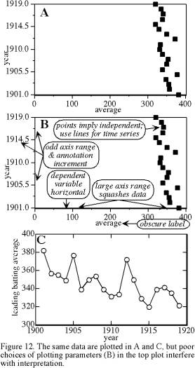
Crossplots can hide or reveal patterns. Plotting technique affects the efficiency of visual pattern recognition. Scientists are accustomed to a suite of plotting conventions, and they may be distracted if asked to look at plots that depart substantially from these conventions. I thank Open University [1970] for reminding me of some of the following plotting hints, which I normally take for granted. Figure 12 illustrates the effect of a few of these factors.
|
|
• Plot the dependent variable (the one whose behavior you hope to predict from the other variable) on the vertical axis, and plot the independent variable on the horizontal axis.
• Choose an aspect ratio for the plot that maximizes information (e.g., if we are examining the changes in Y values throughout a long time series, then the horizontal X axis can be much longer than the vertical Y axis).
• Plot variables with values increasing to the right and upward.
• Choose simple scale divisions, usually with annotated major divisions and with tics for simple subdivisions (e.g., range of 20-40 with annotation interval of 5 and tic spacing of 1).
• Choose a total plot range for each variable that is as small as possible, subject to these two restrictions: simple scale divisions and inclusion of all data points.
• Make an exception to the previous hint by including major meaningful scale divisions such as zero or 100%, only if this inclusion requires a relatively small expansion of the plot range.
• Plot data points as solid or open circles or crosses.
• If more than one dataset is included on the same plot, use readily distinguishable symbols.
• Label each axis with the variable name and its units.
• If data are a time series, connect the points with line segments. If they are independent, fit a line or curve through the data, not connecting line segments.
• If possible, transform one or both variables so that the relationship between them is linear (e.g., choose among linear, semilog, and log-log plots).
Individual scientific specialties routinely violate one or more of the hints above. Each specialty also uses arbitrary unstated conventions for some plotting options:
• whether to frame the plot or just use one annotated
line for each axis;
• whether to use an internal grid or just marginal tics on the frame
or lines;
• whether to put tics on one or both sides, and whether to put them inside
or outside the plot frame.
* * *
Extrapolation and Interpolation:
If a relationship has been established between variables X and Y, then one can predict the value of Yi at a possibly unmeasured value of Xi. The reliability of this prediction depends dramatically on where the new Xi is with respect to the locations of the Xi that established the relationship. Several rules of thumb apply to interpolation and extrapolation:
• interpolation to an Xi location that is between closely spaced previous Xi is relatively safe,
• interpolation between widely spaced previous Xi is somewhat hazardous,
• extrapolation for a short distance (<20% of the range of
the previous Xi) is somewhat
hazardous,
• extrapolation for a great distance is foolhardy, and
• both interpolation and extrapolation are much more reliable when the
relationship is based on independent data than when it is based on non-independent
data such as a time series.
For example, when we saw the pattern of temporal changes in the U.S. deficit, the data appeared to fit a trend of increasing deficit rather well, so one should be able to extrapolate to 1991 fairly reliably. However, extrapolation ability is weaker for a time series than for independent events. As I am typing this, it is January 1991, the U.S. has just gone to war, Savings & Loans are dropping like flies, the U.S. is in a recession, and a deficit as small as the extrapolated value of 22% seems hopelessly optimistic. In contrast, when you read this, the U.S. budget hopefully is running a surplus.
As another example, we have already examined the changes with time of cigarette smoking among high school students, and we concluded that extrapolation from the two points of Figure 11a was foolhardy. With the data from Figure 11b, we might extrapolate beyond 1989 by perhaps 2-3 years and before 1975 by perhaps one year; the difference in confidence between these two extrapolations is due to the better-defined trend for 1983-1989 than for 1976-1980. Because these data are from a time series, any extrapolation is somewhat hazardous: if cigarette smoking were found in 1990 to be an aphrodisiac, the 1983-1989 pattern would immediately become an obsolete predictor of 1990 smoking rates. If there were such a thing as a class of 1986.5, then interpolation for the interval 1983-1989 would be very reliable (error <0.5%), because of extensive data coverage and small variance about the overall trend. In contrast, interpolation of a predicted value for some of the unsampled years in the interval 1975-1980 would have an error of at least 1%, partly because data spacing is larger but primarily because we are unsure how much of the apparent secular change is due to measurement errors. If we knew that the first three measurements (in 1975, 1978, & 1980) constituted random scatter about the same well-defined trend of 1983-1989, then surprisingly it would be more accurate to predict values for these three years from the trend than to use the actual measurements.
|
|
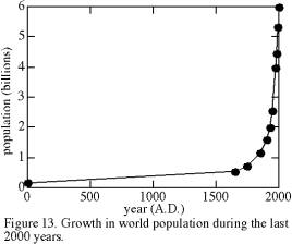
An extreme example of the difference between extrapolation and interpolation for time series is world population (Figure 13). The validity of interpolated population within the last 2000 years depends on how much one trusts the simple pattern of Figure 13. The prolonged gap between 1 A.D. and 1650 conceivably could mask excursions as large as that of 1650-present, yet we know independently from history that such swings have not occurred. The combination of qualitative historical knowledge and the pattern of Figure 13 suggests that even the Black Death, which killed a large proportion of the population, caused less total change than is now occurring per decade. For purposes of defining the trend and for interpolation, then, both the distance between bracketing data points and the rate of change are important. Thus the great increase in sampling density at the right margin of Figure 13 is entirely appropriate, although a single datum at about 1000 A.D. would have lent considerable improvement to trend definition.
Extrapolation of world population beyond the limits of Figure 13 is both instructive and a matter of world concern. Predicting populations prior to 1 A.D. would be based on very scanty data, yet it appears that values would have been greater than zero and less than the 1 A.D. value of 0.2 billion. In contrast, extrapolation of the pattern to future populations suggests that the world population soon will be infinite. Reality intervenes to tell us that it is impossible for the pattern of Figure 13 to continue for much longer.
The three examples above are atypical in that they all are time series -- measurements of temporal changes of a variable. Interpolation, extrapolation, and indeed any interpretation of a time series is ambiguous, because time is an acausal variable. Often one can hypothesize a relationship between two variables that lends confidence to one’s interpretation. In contrast, the source of variations within a time series may be unmeasured and possibly even unidentified.
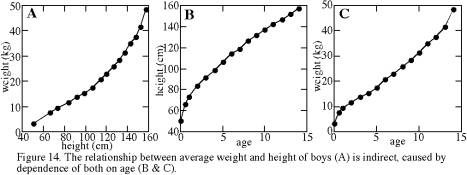
The challenge of avoiding the confounding effect of time is present in all sciences. It is particularly acute within the social sciences, because some variables that might affect human behavior are difficult to hold constant throughout an experiment. For example, consider the relationship between height and weight of boys, shown in Figure 14a. The relationship is nonlinear, and we might be tempted to extrapolate that a 180-cm-high boy could be as much as twice as heavy as a 160-cm-high boy. Clearly neither height nor weight is normally distributed, and in fact it would be absurd to speak of the average height or weight of boys, unless one specified the boys’ age. Figure 14a is actually based on a tabulation for boys of different ages. Age is the causal variable that controls both height and weight and leads to a correlation between the two. Both change systematically but nonlinearly with age (Figures 14b and 14c): early growth is dominantly in height and later growth is dominantly in weight, leading indirectly to the pattern of Figure 14a.
|
|
Time series in particular, and nonindependent sampling in general, jeopardize interpolation and especially extrapolation. Nonlinearities are also a hazard, and we shall explore their impacts more fully in the subsequent section. First, however, let us assume the ideal correlation situation -- independent sampling and a linear relationship. How can we confidently and quantitatively describe the correlation between two variables?
* * *
The type of test appropriate for identifying significant correlations depends on the kind of measurement scale. For classification data, such as male and female responses to an economic or psychological study, a test known as the contingency coefficient searches for deviations of observed from expected frequencies. For ranked, or ordinal, data where relative position along a continuum is known, the rank correlation coefficient is appropriate. Most scientific measurement scales include not just relative position but also measurable distance along the scale, and such data can be analyzed with the correlation coefficient or rank correlation coefficient. This section focuses on analysis of these continuous-scale data, not of classification data.
Suppose that we suspect that variable Y is linearly related to variable X. We need not assume existence of a direct causal relationship between the two variables. We do need to make the three following assumptions: first, that errors are present only in the Yi; second, that these errors in the Yi are random and independent of the value of Xi; and third, that the relationship between X and Y (if present) is linear. Scientists routinely violate the first assumption without causing too many problems, but of course one cannot justify a blunder by claiming that others are just as guilty. The second assumption is rarely a problem and even more rarely recognized as such. The third assumption, that of a linear relationship, is often a problem; fortunately one can detect violations of this assumption and cope with them.
The hypothesized linear relationship between Xi and Yi is of the form: Y = mX+b, where m is the slope and b is the Y intercept (the value of Y when X equals zero). Given N pairs of measurements (Xi,Yi) and the assumptions above, then the slope and intercept can be calculated by linear regression, from:
m = [NΣXiYi-(ΣXi)(ΣYi)]/[NΣXi2-(ΣXi)2]
b = [(ΣYi)(ΣXi2)-(ΣXiYi)(ΣXi)]/[NΣXi2-(ΣXi)2]
Most spreadsheet and graphics programs include a linear regression option. None, however, mentions the implicit assumptions discussed above.
Linear regression fits the line that minimizes the squares of the residuals of Yi deviations from the line. This concept is illustrated in Figure 15a, which shows a linear regression of leading National League batting averages for the years 1901-1920. This concept of minimizing the squares of Yi deviations is very important to remember as one uses linear regression, for it accounts for several characteristics of linear regression.
|
|
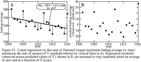
First, we now understand the assumption that only the Yi have errors and that these errors are random, for it is these errors or discrepancies from the trend that we are minimizing. If instead the errors were all in the Xi, then we should minimize the Xi instead (or, much easier, just rename variables so that Y becomes the one with the errors).
Second, minimizing the square of the deviation gives greatest weighting to extreme values, in the same way that extreme values dominate a standard deviation. Thus, the researcher needs to investigate the possibility that one or two extreme values are controlling the regression. One approach is to examine the regression line on the same plot as the data. Even better, plot the regression residuals -- the differences between individual Yi and the predicted value of Y at each Xi, as represented by the vertical line segments in Figure 15a. Regression residuals can be plotted either as a function of Xi (Figure 15b) or as a histogram.
Third, the use of vertical deviations accounts for the name linear regression, rather than a name such as linear fit. If one were to fit a trend by eye through two correlated variables, the line would be steeper than that determined by regression. The best-fit line regresses from the true line toward a horizontal no-fit line with increases of the random errors of Y. This corollary is little-known but noteworthy; it predicts that if two labs do the same type of measurements of (Xi, Yi), they will obtain different linear regression results if their measurement errors are different.
Fitting a linear regression does not imply that the obtained trend is significant. The correlation coefficient (R) measures the degree to which two variables are linearly correlated. We have seen above how to calculate the slope m of what is called the regression of Y on X: Y=mX+b. Conversely, we could calculate the slope m' of regression of X on Y: X=m'Y+b'. Note that we are abandoning the assumption that all of the errors must be in the Yi. If X and Y are not correlated, then m=0 (a horizontal line) and m'=0 (a vertical line), so the product mm'=0. If the correlation is perfect, then m=1/m', or mm'=1. Thus the product mm' provides a unitless measure of the strength of correlation between two variables [Young, 1962]. The correlation coefficient (R) is:
R=(mm')0.5 = [NΣXiYi-(ΣXi)(ΣYi)]/{[NΣXi2-(ΣXi)2]0.5•[NΣYi2-(ΣYi)2]0.5}
The correlation coefficient is always between -1 and 1. R=0 for no correlation, R=-1 for a perfect inverse correlation (i.e., increasing X decreases Y), and R=1 for a perfect positive correlation. What proportion of the total variance in Y is accounted for by the influence of X? R2, a positive number between 0 and 1, gives that fraction.
Whether or not the value of R indicates a significant, or non-chance, correlation depends both on R and on N. Table 7 gives 95% and 99% confidence levels for significance of the correlation coefficient. The test is called a two-tailed test, in that it indicates how unlikely it is that uncorrelated variables would yield either a positive or negative R whose absolute value is larger than the tabulated value. For example, linear regression of federal budget deficits versus time gives a high correlation coefficient of R=0.76 (Figure 9C). This pattern of steadily increasing federal budget deficits is significant at >99% confidence; for N=30, the correlation coefficient only needs to be 0.463 for the 99% significance level (Table 7).
Table 7: 95% and 99% confidence levels for significance of the correlation coefficient [Fisher and Yates, 1963].
|
N: |
3 |
4 |
5 |
6 |
7 |
8 |
9 |
10 |
11 |
12 |
|
R95: |
0.997 |
0.95 |
0.878 |
0.811 |
0.754 |
0.707 |
0.666 |
0.632 |
0.602 |
0.576 |
|
R99: |
1 |
0.99 |
0.959 |
0.917 |
0.874 |
0.834 |
0.798 |
0.765 |
0.735 |
0.708 |
|
N: |
13 |
14 |
15 |
16 |
17 |
18 |
20 |
22 |
24 |
26 |
|
R95: |
0.553 |
0.532 |
0.514 |
0.497 |
0.482 |
0.468 |
0.444 |
0.423 |
0.404 |
0.388 |
|
R99: |
0.684 |
0.661 |
0.641 |
0.623 |
0.606 |
0.59 |
0.561 |
0.537 |
0.515 |
0.496 |
|
N: |
28 |
30 |
40 |
50 |
60 |
80 |
100 |
250 |
500 |
1000 |
|
R95: |
0.374 |
0.361 |
0.312 |
0.279 |
0.254 |
0.22 |
0.196 |
0.124 |
0.088 |
0.062 |
|
R99: |
0.479 |
0.463 |
0.402 |
0.361 |
0.33 |
0.286 |
0.256 |
0.163 |
0.115 |
0.081 |
Table 7 exhibits two features that are surprising. First, although we have already seen that N=2 gives us no basis for separating signal from noise, we would expect that N=3 or 4 should permit us to determine whether two variables are significantly correlated. Yet if N=3 or 4 we cannot be confident that the two variables are significantly correlated unless we find an almost perfectly linear correlation and thus an R of almost 1 or -1. Second, although we might accept that more pairs of (Xi, Yi) points would permit detection of subtler correlations, it is still remarkable that with N>200 a correlation can be significant even if R is only slightly larger than zero. With practice, one can tentatively identify whether two variables are significantly correlated by examining a crossplot, and Figure 16 is provided to aid that experience gathering. With very large N, however, the human eye is less able to identify correlations, and the significance test of Table 7 is much more reliable.
|
|
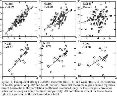
There is an adage: “One doesn’t need statistics to determine whether or not two variables are correlated.” This statement not only ignores scientists’ preference for quantitative rather than qualitative conclusions; it is simply wrong when N is very small or very large. When N is very small (e.g., N<6), the eye sees correlations that are not real (significant). When N is very large (e.g., N>200), the eye fails to discern subtle correlations.
* * *
The biggest pitfall of linear regression and correlation coefficients is that so many relationships between variables are nonlinear. As an extreme example, imagine applying these techniques to the annual temperature variation of Anchorage (Figure 10b). For a sinusoidal distribution such as this, the correlation coefficient would be virtually zero and regression would yield the absurd conclusion that knowledge of what month it is (X) gives no information about expected temperature (Y). In general, any departure from a linear relationship degrades the correlation coefficient.
The first defense against nonlinear relationships is to transform one or both variables so that the relation between them is linear. Taking the logarithm of one or both is by far the most common transformation; taking reciprocals is another. Taking the logarithm of both variables is equivalent to fitting the relationship Y=bXm rather than the usual Y=b+mX. Our earlier plotting hint to try to obtain a linear relationship had two purposes. First, linear regression and correlation coefficients assume linearity. Second, linear trends are somewhat easier for the eye to discern.
A second approach is to use a nonparametric statistic called the rank correlation coefficient. This technique does not require a linear correlation. It does require a relationship in which increase in one variable is accompanied by increase or decrease in the other variable. Thus the technique is inappropriate for the Anchorage temperature variations of Figure 10b. It would work fine for the world population data of Figure 13, because population is always increasing but at a nonlinear rate. To determine the rank correlation coefficient, the steps are:
1) assign a rank to each Xi of from 1 to N,
according to increasing size of Xi;
2) rank the Yi in
the same way;
3) subtract each Xi
rank from its paired Yi rank; we will call this difference in rankings di;
4) determine the rank correlation coefficient r, from
r = 1 - [6(Σdi2)]/[N(N2-1)].
The rank correlation coefficient r is much like the linear correlation coefficient R, in that both have values of -1 for perfect inverse correlation, 0 for no correlation, and +1 for perfect positive correlation. Furthermore, Table 7 above can be used to determine the significance of r in the same way as for R.
For example, the world population data of Figure 13 obviously show a close relationship of population to time. These data give a (linear) correlation coefficient of R=0.536, which is not significant according to Table 7. Two data transforms do yield correlations significant at the 99% confidence level: an exponential fit of the form Y=b+10mx (although this curve fit underestimates current population by more than 50%), and a polynomial fit of the form Y=b+m1X+m2X2 (although it predicts that world population was much less than zero for 30-1680 A.D.!). In contrast, the rank correlation coefficient is r=1.0, which is significant at far more than the 99% confidence level.
Nonlinearities are common; the examples that we have just seen are a small subset. No statistical algorithm could cope with or even detect the profusion of nonlinear relationships. Thus I have emphasized the need to make crossplots and turn the problem of initial pattern recognition over to the eye.
Nonlinearities can be more sudden and less predictable than any of those shown within the previous examples. Everyone knows this phenomenon as ‘the straw that broke the camel's back’; the scientific jargon is ‘extreme sensitivity to initial conditions’. Chaos, a recent physics paradigm, now is finding such nonlinearities in a wide variety of scientific fields, particularly anywhere that turbulent motion occurs. The meteorologist originators of chaos refer to the ‘Butterfly Effect’: today’s flapping of an Amazon butterfly’s wings can affect future U.S. weather. Gleick [1987] gives a remarkably readable overview of chaos and its associated nonlinearities.
Due to extreme nonlinearities, a causal variable can induce a totally different kind of result at low concentration than at high concentration. An example is that nitroglycerin is a common medication for heart problems, yet the patient never explodes! Low concentrations of some causal variables can have surprisingly large effects, through development of a feedback cycle. Such a cycle, for example, is thought to account for the mechanism by which minute oscillations in the earth’s orbit cause enormous fluctuations in global climate known as ice ages and interglacial stages. Extreme nonlinearities are the researcher’s bane.
* * *
• Correlation can describe a relationship, but it cannot establish causality.
• Many variables have secular trends, but the correlation with time is indirect: secular change in a possibly unidentified causal variable causes the measured dependent variable to exhibit secular change.
• Crossplots are the most robust and reliable way to look for a relation between variables.
• Statistical correlation techniques assume independent measurements, so they must be used with caution when measurements are not independent (e.g., time series or grouped data).
• Interpolation between independent measurements is safe, but interpolation between non-independent measurements is risky.
• Extrapolation beyond the range of previous measurements is usually risky.
• Linear regression and the correlation coefficient R assume a linear relationship between variables.
• Examination of regression residuals is needed, to detect systematic mismatches.
• Nonlinearity can complicate relationships among variables enormously.
* * *
“Felix qui potuit rerum cognoscere causas.”
(Happy is he who has been able to learn the causes of things) [Virgil, 70-19
B.C.]
Causality is a foundation of science, but it is not a firm foundation. Our concept of causality has been transformed more than once and it continues to evolve.
During the classical Greek period, to seek causes meant to seek the underlying purposes of phenomena. This concept of causality as purpose is identified with Aristotle, but Aristotle was an advocate rather than an initiator of this focus. The search for underlying purpose is also a religious concern, and the overlap between science and religion was correspondingly greater in ancient Greece than in modern times. Perhaps the religious connotation partly explains the shift away from Aristotelian causality during the last few centuries, but I suspect that the decisive factor was the growing scientific emphasis on verifiability. Greek science felt free to brainstorm and speculate about causes, but modern science demands tests of speculations. Testing purposes is much less feasible than testing modern associative causality. Modern scientific concern about purpose is confined primarily to some aspects of biology and social science. Even most of these questions (e.g., “what is the purpose of brain convolutions?”) refer not to an underlying plan but to function or evolutionary advantage.
Hume [1935] redefined causality in more pragmatic terms. His definition of a cause is “an object precedent and contiguous to another, and where all objects resembling the former are placed in like relations of precedency and contiguity to those objects that resemble the latter.” We can forgive Hume’s constipated wording, I hope, on the grounds that definitions, like legal jargon, must be unambiguous and yet comprehensive. In other words, systematic (nonrandom) proximity in both space and time implies causality, and the event that occurs first is considered to be the cause of the second event. If event B is commonly preceded by an association with event A, then event A is a cause of event B. Note that neither requires the other: A may not be the only type of event that can cause B, and other conditions may be needed before A can cause B. We will consider these variables of causality and their tests in a later section on Mill’s canons.
Lenzen [1938] used the example of Newtonian physics to demonstrate that even Hume’s careful definition has exceptions. Cause does not always precede effect, as is evidenced by the fact that force causes simultaneous acceleration, not delayed acceleration. Cause and effect need not be contiguous, as is evidenced by the fact that gravitational attraction acts over millions of miles (else the earth would go careening away from the sun and off into space). To me, these exceptions are inconsequential. Hume’s causality is meant to be a pragmatic concept, and a principle that is almost always useful should not be discarded for the purity of a void.
If causality is to be limited to the observable and testable as Hume’s concept is, then several familiar attributes of causality may have to be stripped away: Aristotelian interest in purpose, the inevitability or necessity of an effect given a cause, and concern with underlying (unobservable) mechanisms [Boyd, 1985]. We are left with a sterile association between events, firmly founded in observations but lacking deeper understanding of processes. One twentieth-century philosophical school reached a similar conclusion with different logic: causality is nonunique -- one ‘cause’ can generate several paths and different causes can lead to the same ‘effect’ -- so causality should be confined to associations. Physicist Victor Weisskopf often said that causality is simply connections. A philosophical movement called logical positivism skirted this limitation by emphasizing that deduction from natural laws can provide a causal explanation of observations.
For the Sufis, cause-and-effect is a misguided focus on a single thread in the tapestry of intertwined relationships. They illustrate this lesson with the parable of the hanged man [Shah, 1972], which we can recast as follows:
In 212 B.C., in his home in Syracuse, while working a math problem, Archimedes was killed by a Roman soldier. What caused his death? Was it that his applied scientific contributions in the form of novel defensive weapons were no defense against treason? Was it that the leader of the victorious invaders, in giving the order to leave the house of Archimedes alone, failed to assure that individual soldiers attended to the order? Was it that Archimedes, when commanded by a soldier to leave his home, was so preoccupied by his math problem that he refused to let even the fall of a city distract him? Or was it simply that the soldier had had a hard day, exhausting his patience for the cranky stubbornness of an old man?
* * *
Causality or pattern is the choice a cultural one rather than innate? And if it is cultural, what about related fundamental scientific assumptions: comparison, linear thought, and time? A provocative perspective on these questions was provided by Lee’s [1950] classic study of the language of the Trobriand Islanders, a virtually pristine stone-age culture of Southeast Asia. Her goals were to extract both cultural information and fundamental insights into their thought patterns and “codification of reality”. She did not assume that reality is relative; she did assume that different cultures can categorize or perceive reality in different ways, and that language provides clues to this perceptual approach.
The Trobriand language has no adjectives; each noun contains a suite of implicit attributes, and changing an attribute changes the object or noun. The Trobriand language has no change, no time, no distinction between past and present. Lacking these, it also lacks a basis for causality, and indeed there is no cause-and-effect. Absences of adjectives, change, and time distinctions are aspects of a broader characteristic: the virtual absence of comparisons of any kind in Trobriand language or world-view. There is no lineal connection between events or objects.
The Trobriand culture functions well without any of these traits that we normally consider essential and implicit to human perception. So implicit are these assumptions that Bronislaw Malinowski studied the Trobriand Islanders without detecting how fundamentally different their world-view is. Not surprisingly, he was sometimes frustrated and confused by their behavior.
The Trobriand people use a much simpler and more elegant perceptual basis than the diverse assumptions of change, time distinctions, causality, and comparison. They perceive patterns, composed of “a series of beings, but no becoming” or temporal connection. When considering a patterned whole, one needs no causal or temporal relationships; it is sufficient merely to identify ingredients in the pattern.
“Trobriand activity is patterned activity. One act within this pattern brings into existence a pre-ordained cluster of acts… pattern is truth and value for them; in fact, acts and being derive value from the embedding pattern… To him value lies in sameness, in repeated pattern, in the incorporation of all time within the same point.” [Lee, 1950]
During the last 12,000 years an ice age has waned, sea levels have risen, and climates have changed drastically. Plant and animal species have been forced to cope with these changes. Since the development of agriculture about 12,000 years ago, human progress has been incredibly fast. Biological evolution cannot account for such rapid human change; cultural evolution must be responsible. Perhaps the Trobriand example lends some insight into these changes. A Trobriandesque world-view, emphasizing adherence to pattern, might have substantial survival value in a stable environment. In contrast, climatic stress and changing food supplies favored a different world-view involving imagination and choice. Only in rare cases, such as the Trobriand tropical island, was the environment stable enough for a Trobriand-style perspective to persist.
The Trobriand world-view is in many ways antipodal to that upon which scientific research is based. Yet it is valid, in the same sense that our western world-view is valid: it works (at least in a stable environment). And the viability of such an alien perspective forces us to recognize that some of our fundamental scientific assumptions are cultural: our concepts of causality, comparison, and time may be inaccurate descriptions of reality.
* * *
Scientific causality transcends all of these restricted concepts of causality. It does not abandon concern with inevitability or with underlying mechanisms. Instead it accepts that description of causal associations is intrinsically valid, while seeking fundamental conceptual or physical principles that explain these associations.
Different sciences place different emphases on causality. The social sciences in general give a high priority to identifying causal relationships. Physical sciences often attempt to use causality as a launching point for determining underlying theoretically-based quantitative relationships. Possibly this difference reflects the greater ease of quantifying and isolating variables in the physical sciences. Such sweeping generalizations are simplistic, however -- economics is an extremely quantitative social science.
All concepts of cause-and-effect assume that identical sets of initial conditions yield identical effects. Yet, quantum mechanics demonstrates that this fundamental scientific premise is invalid at the scale of individual atoms. For example, radioactive decay is intrinsically unpredictable for any one atom. If certainty is impossible at the atomic level, the same must be true for larger-scale phenomena involving many atoms. Werner Heisenberg, a champion of atomic-scale indeterminacy, carried this logic to a conclusion that sounds almost like a death knell for causality [Dillard, 1974]: “method and object can no longer be separated. The scientific world-view has ceased to be a scientific view in the true sense of the word.”
Some non-scientists have seized on Heisenberg’s arguments as evidence of the inherent limitations of science. Heisenberg’s indeterminacy and the statistical nature of quantum mechanics are boundary conditions to causal description of particle physics, but not to causal explanation in general. Particle physicists emphasize that virtual certainty can still be obtained for larger-scale phenomena, because of the known statistical patterns among large numbers of random events. The pragmatic causality of scientists finds atomic indeterminacy to be among the least of its problems. Far more relevant is the overwhelming complexity of nature. Heisenberg may have shaken the foundations of science, but few scientists other than physicists felt tremors in the edifice.
It seems that a twentieth-century divergence is occurring, between theoretical concepts of causality and the working concepts used by scientists. One can summarize the differences among these different concepts of causality, using the following symbols:
A is the cause,
B is the effect,
⇒ means ‘causes’,
≠> means ‘does not necessarily cause’,
∴ means ‘therefore’,
Ai is an individual observation of A, and
![]() is average behavior of A.
is average behavior of A.
The different concepts of causality are then:
Sufi and Trobriand patterns: … . A, B, … .
Aristotle: A⇒B, in order to …
Hume: If A, then B; or A, ∴B
logical positivist: theory C predicts ‘A, ∴B’, & observation
confirms it
Quantum mechanics: Ai ≠> Bi, yet ![]() =>
=>![]()
scientific consensus: If A, then probably B, possibly because … .
Scientists’ working concept of causality remains unchanged, effectively useful, and moderately sloppy: if one event frequently follows another, and no third variable is controlling both, then infer causality and, if feasible, seek the underlying physical mechanism. Ambiguities in this working concept sometimes lead to unnecessary scientific debates. For example, the proponent of a causal hypothesis may not expect it to apply universally, whereas a scientist who finds exceptions to the hypothesis may announce that it is disproved.
* * *
The logician’s concept of causality avoids the ambiguity of the scientist’s concept. Logicians distinguish three very different types of causality: sufficient condition, necessary condition, and a condition that is both necessary and sufficient.
If several factors are required for a given effect, then each is a necessary condition. For the example of Archimedes’ death, both successful Roman invasion and his refusal to abandon his math problem were necessary conditions, or necessary causal factors. Many necessary conditions are so obvious that they are assumed implicitly. If only one factor is required for a given effect, then that factor is a sufficient condition. If only one factor is capable of producing a given effect, then that factor is a necessary and sufficient condition. Rarely is nature simple enough for a single necessary and sufficient cause; one example is that a force is a necessary and sufficient condition for acceleration of a mass.
Hurley [1985] succinctly describes the type of causality with which the scientist often deals:
“Whenever an event occurs, at least one sufficient condition is present and all the necessary conditions are present. The conjunction of the necessary conditions is the sufficient condition that actually produces the event.”
For the most satisfactory causal explanation of a phenomenon, we usually seek to identify the necessary and sufficient conditions, not a single necessary and sufficient condition. Often the researcher’s task is to test a hypothesis that N attributes are needed (i.e., both necessary and sufficient) to cause an effect. The scientist then needs to design an experiment that demonstrates both the presence of the effect when the N attributes are present, and the absence of the effect whenever any of these attributes is removed.
Sometimes we cannot test a hypothesis of causality with such a straightforward approach, but the test is nevertheless possible using a logically equivalent statement of the problem. The following statements are logically equivalent [Hurley, 1985], regardless of whether A is the cause and B is the effect or vice versa (with -A meaning ‘not-A’ and ≡ meaning ‘is equivalent to’):
A is a necessary condition for B
≡ B is a sufficient condition for A
≡ If B, then A (i.e., B, ∴A)
≡ If A is absent, then B is absent (i.e., -A, ∴-B)
≡ Absence of A is a sufficient condition for the absence of B
≡ Absence of B is a necessary condition for absence of A.
* * *
Mill’s Canons: Five Inductive Methods
John Stuart Mill [1930], in his influential book System of Logic, systematized inductive techniques. The results, known as ‘Mill's Canons’, are five methods for examining variables in order to identify causal relationships. These techniques are extremely valuable and they are routinely used in modern scientific experiments. They are not, however, magic bullets that invariably hit the target. The researcher needs to know the strengths and limitations of all five techniques, as each is most appropriate only in certain conditions.
A little jargon will aid in understanding the inductive methods. Antecedent conditions are those that ‘go before’ an experimental result; antecedent variables are those variables, known and unknown, that may affect the experimental result. Consequent conditions are those that ‘follow with’ an experimental result; consequent variables are those variables whose values are affected by the experiment. In these terms, the inductive problem is expressed as seeking the antecedent to the consequent of interest, i.e., seeking the causal antecedent. In considering the inductive methods, a useful shorthand is to refer to antecedent variables with the lower-case letters a, b, c, … and to refer to consequent variables with the upper-case letters Z, Y, X, …
Mill’s Canons bear 19th-century names, but the concepts are familiar to ancient and modern people in less rigorous form:
a must cause Z, because:
• whenever I see Z, I also find a (the method of agreement);
• if I remove a, Z goes away (the method of difference);
• whether present or absent, a always accompanies Z (the joint method of agreement and difference);
• if I change a, Z changes correspondingly (the method of concomitant variations);
• if I remove the dominating effect of b on Z, the residual Z variations correlate with a (the method of residues).
Each of the five inductive methods has strengths and weaknesses, discussed below. The five methods also share certain limitations, which we will consider first.
Mill was aware that association or correlation does not imply causality, regardless of inductive method. For example, some other variable may cause both the antecedent and consequent (h⇒c, h⇒Z, ∴ c correlates with Z, but c≠>Z). Thus Mill would expand the definition of each method below, ending each with an escape clause such as “or the antecedent and result are connected through some fact of causation.” In contrast, I present Mill’s Canons as methods of establishing relationships; whether the relationships are directly causal is an independent problem.
When we speak of a causal antecedent, we usually think of a single variable. Instead, the ‘causal antecedent’ may be a conjunction of two or more variables; we can refer to these variables as the primary and facilitating variables. If we are aware of the facilitating variables, if we assure that they are present throughout the experiment, and if we use the inductive methods to evaluate the influence of the primary variable, then success with Mill’s Canons is likely. If we are unaware of the role of the facilitating variables, if we cannot turn them on and off at will, or if we cannot measure them, then we need a more sophisticated experimental design.
If several different experiments yield the same result, and these experiments have only one factor (antecedent) in common, then that factor is the cause of the observed result. Symbolically, abc⇒Z, cde⇒Z, cfg⇒Z, ∴c⇒Z; or abc⇒ZYX, cde⇒ZW, cfg⇒ZVUT, ∴c⇒Z. The method of agreement is theoretically valid but pragmatically very weak, for two reasons:
• almost never can we be certain that the various experiments share only one common factor. We can increase confidence in the technique by making the experiments as different as possible (except of course for the common antecedent), thereby minimizing the risk of an unidentified common variable; and
• some effects can result from two independent causes, yet this method assumes that only one cause is operant. If two or more independent causes produce the same experimental result, the method of agreement will incorrectly attribute the cause to any antecedent that coincidentally is present in both experiments. Sometimes the effect must be defined more specifically and exclusively, so that different causes cannot produce the same effect.
It is usually safest to restate the method of agreement as: if several different experiments yield the same result, and these experiments appear to have only one antecedent factor in common, then that factor may be the cause of the observed result. Caution is needed, to assure that the antecedent and result are not both controlled by some third variable, that all relevant factors are included, and that the effect or result is truly of the same kind in all experiments. Time is a variable that often converts this method into a pitfall, by exerting hidden control on both antecedents and results. Ideally, the method of agreement is used only to spot a possible pattern, then a more powerful experimental design is employed to test the hypothesis.
If a result is obtained when a certain factor is present but not when it is absent, then that factor is causal. Symbolically, abc⇒Z, ab⇒Z, ∴c⇒Z; or abc⇒ZYXW, ab⇒YXW, ∴c⇒Z. The method of difference is scientifically superior to the method of agreement: it is much more feasible to make two experiments as similar as possible (except for one variable) than to make them as different as possible (except for one variable).
The method of difference has a crucial pitfall: no two experiments can ever be identical in all respects except for the one under investigation. Thus one risks attributing the effect to the wrong factor. Consequently, almost never is the method of difference viable with only two experiments; instead one should do many replicate measurements.
The method of difference is the basis of a powerful experimental technique: the controlled experiment. In a controlled experiment, one repeats an experiment many times, randomly including or excluding the possibly causal variable ‘c’. Results are then separated into two groups -- experiment and control, or c-variable present and c-variable absent -- and statistically compared. A statistically significant difference between the two groups establishes that the variable c does affect the results, unless:
• the randomization was not truly random, permitting some other variable to exert an influence; or
• some other variable causes both c and the result.
During his long imprisonment, the scientist made friends with a fly and trained it to land on his finger whenever he whistled. He decided to carry out a controlled experiment. Twenty times he whistled and held out his finger; every time the fly landed there. Then he pulled off the fly’s wings. Twenty times he whistled and held out his finger; not once did the fly land there. He concluded that flies hear through their wings.
Joint Method of Agreement and Difference
If a group of situations has only one antecedent in common and all exhibit the same result, and if another group of similar situations lacks that antecedent and fails to exhibit the result, then that antecedent causes the result. Symbolically, abc⇒ZYX, ade⇒ZWV, and afg⇒ZUT; bdf⇒YWU and bceg⇒XVT, ∴a⇒Z.
This method is very similar to the methods of agreement and of difference, but it lacks the simple, simultaneous pairing of presence or absence between one antecedent and a corresponding result. Effectively, this method treats each ‘situation’ or experiment as one sample in a broader experiment demonstrating that whenever a is present, Z results, and whenever a is absent, Z is absent. The method makes the seemingly unreasonable assumption of ‘all other things being equal’; yet this assumption is valid if the experiment is undertaken with adequate randomization.
Method of Concomitant Variations
If variation in an antecedent variable is associated systematically with variation in a consequent variable, then that antecedent causes the observed variations in the result. Symbolically, abc⇒Z, abΔc⇒ΔZ, ∴c⇒Z; or abc⇒WXYZ, abΔc⇒WXYΔZ, ∴c⇒Z.
The method of concomitant variations is like a combination of the methods of agreement and difference, but it is more powerful than either. Whereas the methods of agreement or difference merely establish an association, the method of concomitant variations quantitatively determines the relationship between causal and resultant variables. Thus the agreement and difference methods treat antecedents and consequents as attributes: either present or absent. The method of concomitant variations treats them as variables.
Usually one wants to know whether a relationship is present, and if so, what that relationship is. This method simultaneously addresses both questions. Furthermore, nonlinear relationships may fail the method of difference but be identified by the method of concomitant variation. For example, a method-of-difference test of the efficacy of a medication might find no difference between medicated and unmedicated subjects, because the medicine is only useful at higher dosages.
A quantitative relationship between antecedent and result, as revealed by the method of concomitant variation, may provide insight into the nature of that relationship. It also permits comparison of the relative importance of various causal parameters. This technique, however, is not immune to two limitations of the two previous methods:
• determination that a significant relationship exists
does not prove causality; and
• other variables must be prevented from
confounding the result. If they cannot be kept constant, then their potential
biasing effect must be circumvented via randomization.
The correlation techniques described earlier in this chapter exploit the method of concomitant variations.
If one or more antecedents are already known to cause part of a complex effect, then the other (residual) antecedents cause the residual part of the effect. Symbolically, abc⇒WXYZ, ab⇒WXY, ∴c⇒Z.
As defined restrictively above, this method is of little use because it assumes that every potentially relevant antecedent is being considered. Yet a pragmatic method of residues is the crux of much empirical science: identify the first-order causal relationship, then remove its dominating effect in order to investigate second-order and third-order patterns.
The method of residues provided a decisive confirmation of Einstein’s relativity: the theory accurately predicted Mercury’s orbit, including the residual left unexplained by Newtonian mechanics. Another example is the discovery of Neptune, based on an analysis of the residual perturbations of the orbit of Uranus. Similarly, residual deviations in the orbits of Neptune and Uranus remain, suggesting the existence of a Planet X, which was sought unsuccessfully with Pioneer 10 and is still being looked for [Wilford, 1992b].
The archaeological technique of sieving for potsherds and bone fragments is well known. Bonnichsen and Schneider [1995], however, have found that the fine residue is often rich in information: hair. Numerous animal species that visited the site or were consumed there can be identified. Human hair indicates approximate age of its donor and dietary ratio of meat to vegetable matter. Furthermore, it can be radiocarbon dated and may even have intact DNA.
* * *
The five inductive methods establish apparent causal links between variables or between attributes, but they are incomplete and virtually worthless without some indication of the confidence of the link. Confidence requires three ingredients:
• a quantitative or statistical measure of the strength of relationships, such as the correlation statistics described earlier in this chapter;
• discrimination between causal correlation and other sources of correlation, which is the subject of the next section; and
• an understanding of the power or confirmation value of the experiment, a subject that is discussed in Chapter 7.
The five inductive methods differ strikingly in confirmatory power. The Method of Difference and the Method of Concomitant Variations are the most potent, particularly when analyzed quantitatively with statistics. The Method of Agreement is generally unconvincing. Unfortunately, an individual hypothesis usually is not amenable to testing by all five methods, so one may have to settle for a less powerful test. Sometimes one can recast the hypothesis into a form compatible with a more compelling inductive test.
* * *
Causality needs correlation; correlation does not need causality. The challenge to scientists is to observe many correlations and to infer the few primary causalities.
Mannoia [1980] succinctly indicates how direct causal relationships are a small subset of all observed correlations. Observed statistical correlations (e.g., between A and B) may be:
• accidental correlations (1 of 20 random data comparisons
is ‘significant’ at the 95% confidence level);
• two effects of a third variable that is causal and possibly unknown
(X⇒A & X⇒B);
• causally linked, but only indirectly through intervening factors (A⇒X1⇒X2⇒B,
or B⇒X1⇒X2⇒A);
or
• directly causally related (A⇒B
or B⇒A).
Earlier in this chapter, we examined quantitative measures of correlation strength and of the significance of correlations. Only an inductive conceptual model, however, can provide grounds for assigning an observed correlation to one of the four categories of causality/correlation. No quantitative proof is possible, and the quantitative statistical measures only provide clues.
Many factors affect or ‘cause’ change in a variable. Usually, our interest in these factors decreases with decreasing strength of correlation between the causal variables Ai and the effect B. In general, we judge the relative importance of various causal variables based on two factors: the strength of correlation and the rate of change dB/dAi. High correlation strength means that much of the observed variation in effect B is somehow accounted for by variation in possible causal variable Ai. High rate of change means that a substantial change in effect B is associated with a modest change in causal variable Ai. However, rate of change alone can be misleading, for the total natural range of two causal variables A1 and A2 may be so different that dB/dA1 could be larger than dB/dA2 and yet A2 causes more variation in B than A1 does. Earlier in this chapter, we employed the correlation coefficient as a quantitative measure of correlation strength and the linear-regression slope as a measure of rate of change.
If one has three variables (C, D, and E) that are correlated, correlation strength can be used to infer likely relationships among them. Statistical techniques such as path analysis and analysis of covariance are best for determining these interconnections, but we will confine the present discussion to a more qualitative consideration of the problem. For example, suppose the correlation strengths among C, D, and E are as follows: C/D strong, D/E strong, and C/E weak. Probably, the weak relationship C/E is a byproduct of the two stronger correlations C/D and D/E, each of which may be causal. Direct causal connections (A=>B) usually generate much stronger correlations than indirect ones (A⇒X1⇒X2⇒B). Extraneous factors affect each of the steps (A⇒X1, X1⇒X2, and X2⇒B) of the indirect correlation, thus weakening the overall correlation between A and B. Note, however, that relative strengths of correlations cannot establish causality; they only provide evidence about relative proximity of links among variables. For example, the pattern of C/D strong, D/E strong, and C/E weak could result either from C⇒D⇒E or from E⇒D⇒C.
Many surveys of U.S. voting patterns have shown that those who vote Republican have, on average, more education than Democratic voters. Does this mean that education instills Republican voting, or perhaps that higher intelligence inspires both greater education and Republican voting? Hoover [1988] uses this example to illustrate how social sciences need to beware of correlations induced by an unidentified third variable. More detailed and well-controlled surveys demonstrate that family wealth is the third variable: children of wealthier families tend to acquire a higher level of education and to be wealthier than average, and the voting pattern of wealthier individuals is more likely to be Republican than Democratic.
* * *
The following two examples illustrate the challenge of identifying the causality that manifests as correlation: the investigators had to design experiments to tease out this causal pattern. In both examples, epidemiological studies of a large population were used to identify a statistical association between a pair of variables.
What is the effect of electromagnetic radiation on health? In one study, pregnant women who used video terminals more than 20 hours per week had twice as many miscarriages as did other kinds of female office workers. The authors of the study cautioned, however, that radiation was not necessarily the cause of this difference. For example, the video-intensive jobs might be more stressful.
A statistical study of Denver children found that those who had lived near power-distribution lines were twice as likely to get cancer than other children. This study was criticized for its uncontrolled variables, so other investigators conducted a follow-up study designed to be much better controlled and more diagnostic. Contrary to the researchers’ expectations, the new result was virtually the same as the original, so many scientists concluded that electromagnetic radiation really does seem to affect health. Note the origin of this change in opinions: the combination of a recognizably skeptical scientist and a tighter experiment [Stevens, 1992b].
Compelling scientific evidence is required, because of the potentially staggering human and economic impacts if a causal link between electromagnetic radiation and health were confirmed. A synthesis of more than one hundred studies demonstrates that health impacts are generally negligible [Derry, 1999], but scientific concerns persist, particularly regarding possible long-term effects of cell phones.
Is there a genetic predisposition to alcoholism? Research on this question exemplifies the problem of distinguishing between acquired and inherited characteristics. One of the most successful ways to attack such problems is by studying adopted children. For example, 30-40% of adopted children of alcoholics become alcoholics, compared to only 10% of the general population. This result constitutes good evidence for a genetic origin, but only because it was confined to children of alcoholic fathers; it is conceivable that an alcoholic mother could pass along an acquired dependence to her fetus, as occurs with heroin.
In a different type of experiment, H. Begleiter found a much higher incidence of certain deficiencies in thinking and remembering among alcoholics than among nonalcoholics. Some of these deficiencies disappeared after the subjects stopped drinking, but others persisted for years. Was this evidence of permanent damage caused by alcohol? The author considered a radical alternative hypothesis: instead of the brain deficiency being caused by drinking, it preceded the drinking and was a trait among those most likely to become alcoholics. In studies of children, he found that 30-35% of the sons of alcoholic fathers had the deficiency, although only 1% of a control group did [Kolata, 1992a].
Rare scientists (e.g., Bauer, 1994) claim that the continuing debates about acquired vs. inherited characteristics illustrate deficiencies of sociology. Many non-scientists interpret the debates as revealing the fallibility of scientists. Instead, this research exemplifies the inductive ingenuity of those scientists who can recognize the possibility of a pattern among incredible complexity, then design a test that successfully isolates the primary variables.